President’s Malaria Initiative (PMI)

malaria
epidemiology
country-level
annual
PMI collaborates closely with partner countries to scale up proven interventions and strengthen local capacity and health systems.
Published

October 25, 2024

About the data

The U.S. Government’s focal point for the global fight against malaria, the U.S. President’s Malaria Initiative has helped save millions of lives and contributed to substantial gains in education, productivity, and economic development. PMI started as a five-year initiative with the goal of reducing malaria deaths by 50% in 15 African countries. Thanks to the bipartisan support of Congress and the generosity of the American people, PMI now works in 24 partner countries in sub-Saharan Africa and three programs in the Greater Mekong Subregion in Southeast Asia–representing about 90% of the global malaria burden. PMI delivers cost-effective, life-saving malaria interventions alongside catalytic technical and operational assistance to equip and empower partner countries to end malaria.

Accessing the data

Information on PMI’s life-saving malaria interventions and operational support to partner countries is available on the PMI website

• Under the “Where We Work” tab from the website, fact sheets for the 27 partner countries can be accessed in PDF format. You can right click on the country’s name to access the country’s fact sheet, yearly Malaria Operational Plans and download them.

• Under the “Impact” tab, data on malaria burden, PMI funding, PMI commodity investment and the program’s impact across partner countries are presented through an interactive map or illustrative graph. This map allows users to hover over individual countries to access detailed information on malaria cases, deaths, and associated metrics. Aside this, filters are also available to select the region or the country and sliders to select the year.

• In the “Resources” section, annual reports, comprehensive one-year Malaria Operational Plans (MOPs), technical documents, and reports detailing interventions in each partner country by year are available for download in PDF format. A search can be refined through the use of filters. The filters are for Technical areas, countries and dates.

What does the data look like?

The data are provided for each country on an annual basis and can be accessed through an interactive map or graphical representations. However, no downloadable Excel or CSV files are available. Users must manually extract the data from the map or graph in order to generate Excel or CSV files, should they wish to conduct analyses beyond those available on the website. The following examples illustrate the provided information.

Key points to consider

On the PMI’s website, the data are provided for each country on an annual basis and can be accessed through an interactive map or graphical representations.

  • The data is sourced mostly from the World Malaria Report (WMR)

  • Download Options: There are no downloadable Excel or CSV files available.

  • Manual Data Extraction: Users need to manually extract data from the map or graph to create Excel or CSV files for further analysis.

  • Yearly data might overlook the seasonal trends in malaria transmission, which are affected by variables like rainfall, temperature, and vectors abundance. This can result in either an overestimation or underestimation of the disease burden and the effectiveness of interventions.

  • Behavioral Changes: Changes in population behaviors, such as increased mobility, changes in agricultural practices, or urbanization, can influence transmission dynamics but may not be captured in annual data.

How to use this data

Show the code
# Load packages ####
library(readxl)
library(tidyverse)
── Attaching core tidyverse packages ──────────────────────── tidyverse 2.0.0 ──
✔ dplyr     1.1.4     ✔ readr     2.1.5
✔ forcats   1.0.0     ✔ stringr   1.5.1
✔ ggplot2   3.5.1     ✔ tibble    3.2.1
✔ lubridate 1.9.3     ✔ tidyr     1.3.1
✔ purrr     1.0.2     
── Conflicts ────────────────────────────────────────── tidyverse_conflicts() ──
✖ dplyr::filter() masks stats::filter()
✖ dplyr::lag()    masks stats::lag()
ℹ Use the conflicted package (<http://conflicted.r-lib.org/>) to force all conflicts to become errors
Show the code
library(reshape2)

Attaching package: 'reshape2'

The following object is masked from 'package:tidyr':

    smiths
Show the code
source(here::here("theme_health_radar.R"))

Annual malaria incidence in different countries over time can be easily visualised using line plots. The points plotted at each data point help to communicate that these are annual data, rather than continuous.

Show the code
incidence_pmi <- read_excel("data/malaria_incidence_PMI.xlsx")

# Reshape the data from wide to long format
incidence_long <- incidence_pmi |>
  pivot_longer(cols = -Country, names_to = "Year", values_to = "Incidence") |>
  mutate(Year = as.numeric(Year))  # Convert Year to numeric for plotting

# Convert 'Incidence' to numeric
incidence_long$Incidence <- as.numeric(as.character(incidence_long$Incidence))

# Create a ggplot object with incidence_long data
ggplot(incidence_long, aes(x = Year, y = Incidence, color = Country, group = Country)) +
  # Add lines connecting data points for each country
  geom_line() +
  # Add points at each data point for each country
  geom_point() +
  # Customize the x-axis to show every year in the data range
  scale_x_continuous(breaks = min(incidence_long$Year):max(incidence_long$Year)) + 
  # Customize the y-axis to show breaks from 0 to 400 in increments of 50
  scale_y_continuous(breaks = seq(0, 400, 50)) + 
  # Apply a custom theme 
  theme_health_radar() +
  # Apply a custom color scale 
  scale_colour_manual_health_radar() +  
  # Rotate x-axis text labels 45 degrees and adjust horizontal justification
  theme(axis.text.x = element_text(angle = 45, hjust = 0.5)) +
  # Add labels and title to the plot
  labs(
    title = "Annual malaria incidence (2009-2022)",
    x = "Year",
    y = "Incidence (per 1000 people)",
    colour = "Country",
    # Add a caption with wrapped text for better readability
    caption = str_wrap("The annual malaria incidence (per 1000 people) in Angola, Mozambique, Zambia, and Zimbabwe from 2008 to 2022. Mozambique consistently shows the highest incidence, with a slight decline over the years, stabilizing at around 320 cases per 1000 people by 2022. Zambia’s incidence initially increases until 2014, after which it starts to decline. In Angola, malaria incidence shows an initial decline from 2009 to 2012, followed by a steady rise peaking in 2021, indicating a worsening malaria burden over time. Zimbabwe shows the lowest malaria incidence, marked by significant variability, with the lowest values seen after 2020. These trends highlight differing malaria control progress and challenges across the four countries. Source: World Malaria Report", width = 85)
  )

A paired bar plot is used to compare ITN usage in children under 5 in various countries, before and after PMI implementation.

Show the code
coverage_itn <- read_excel("data/nets_under5_PMI.xlsx")

# Reshape the data for ggplot
coverage_itn_melted <- melt(coverage_itn, id.vars = "Country", variable.name = "Type", value.name = "Percentage")

# Create a ggplot object with coverage_itn_melted data
ggplot(coverage_itn_melted, aes(x = Country, y = Percentage, fill = Type)) +
  # Add bar plots with identity stat and dodge position for side-by-side bars
  geom_bar(stat = "identity", position = position_dodge()) +
  # Apply a custom theme 
  theme_health_radar() +
  # Apply a custom fill scale 
  scale_fill_manual_health_radar() +
  # Add labels and title to the plot
  labs(
    title = "ITN usage among children under 5",
    x = "",  # No label for the x-axis
    y = "Percentage (%)",
    # Add a caption with wrapped text for better readability
    caption = str_wrap("The baseline and endline percentage Insecticide Treated Net (ITN) usage among children under 5 living in Angola, Mozambique, Zambia, and Zimbabwe. The baseline percentage indicates the ITN usage by children under 5 prior to the implementation of the President's Malaria Initiative (PMI), while the endline percentage indicates ITN usage in children under 5 after the implementation of the PMI. Zambia shows the highest endline percentage of ITN coverage, with a significant increase from the baseline. Mozambique shows the most pronounced increase from the baseline. Angola exhibits a relatively small increase in the percentage use of ITNs by children under 5. Source: World Malaria Report", width = 90),
    fill = ""  # No label for the fill legend
  )

The percentage of women receiving Intermittent Preventative Treatment in pregnancy (IPTp) in various countries is represented using a simple bar plot.

Show the code
# Define a single colour for the plot
single_color <- "#1b9e77"

coverage_iptp <- read_excel("data/IPTP_coverage_PMI.xlsx")

# Create a ggplot object with coverage_iptp data
ggplot(coverage_iptp, aes(x = Country, y = Percentage)) +
  # Add bar plots with identity stat and a single fill color
  geom_bar(stat = "identity", fill = single_color) +
  # Apply a custom theme 
  theme_health_radar() +
  # Add labels and title to the plot
  labs(
    title = "Percentage of women receiving IPTp",
    y = "Percentage (%)",
    x = "",  # No label for the x-axis
    # Add a caption with wrapped text for better readability
    caption = str_wrap("The percentage of women receiving Intermittent Preventative Treatment in pregnancy (IPTp) in Angola, Mozambique, Zambia and Zimbabwe. Zambia exhibits the highest coverage, while the other countries have less than 30% of women receiving IPTp. Source: World Malaria Report", width = 100)
  )

How can this data be used in disease modelling?

The data available on the PMI website is valuable for malaria modelling in several ways. It includes indicators that can help in predicting the spread of malaria, assessing the impact of interventions, or understanding regional differences in malaria dynamics. Below are some of the indicators:

  • Estimated malaria incidence per year in each of the partner countries

  • Estimated malaria mortality rate per year in each of the partner countries

  • Percentage of children under 5 who slept under a long-lasting insecticide treated net (LLIN) the night before the survey before and after PMI’s intervention

  • Percentage of pregnant women who received at least three doses of preventive treatment during their last pregnancy before and after PMI’s intervention

  • PMI’s funding in each country.

In the simple example below, we obtain data on Intermittent preventive treatment of malaria during pregnancy (IPTp) access and usage rates in Angola, and assess the impact of these intervention on malaria cases. IPTp is intended to prevent malaria infection by providing pregnant women with three doses of an artemisinin-based combination therapy (ACT). In turn, this prevents risks associated with pregnancy-related complications caused by malaria infection, such as maternal anemia and low birth weights.

Model assumptions

  • The total population size remains constant over time and mosquito populations are asusmed to be at equilibrium.

  • Based on the data obtained from PMI, 19% of women are receiving IPTp in Angola. After three years we incorporate a potential policy change that increases coverage to 50 and/or 70%, respectively.

  • All IPTp doses are completed and the intervention is 100% effective. IPTp reduces the likelihood of infection and further infectiousness, and also shortens the time to recovery after an infection.

  • 0.02% of the Angolan population are women of reproductive age WHO data.

  • The fertility rate \(f\) is defined as the average number of births per woman over her lifetime. The average childbearing years span from 15 to 45 years of age. \(f\) is assumed to be constant over time, and applies uniformly to all susceptible women.

Force of infection

The force of infection is typically expressed in terms of the number of new infections per susceptible individual per unit of time. It is often represented as a function of various factors, including malaria transmission dynamics, the prevalence of infection within the population, and specific interventions aimed at reducing transmission. In this example, the force of infection includes a seasonal forcing function, and current coverage levels of IPTp. For a more detailed explanation of seasonal forcing and the impact of weather dynamics on malaria transmission, please see the Climate Research Unit Timeseries (CRU TS) page. This example also extends other models on this website by demonstrating three scenarios of IPTp coverage.

Show the code
# Load packages ####
library(deSolve)
library(tidyverse)


# Time points for the simulation
Y = 10 # Years of simulation
times <- seq(0, 365*Y, 1)

# Define the SEIR-like model for malaria with time-varying IPTp coverage
iptpmodel <- function(t, x, parms)  {
  with(as.list(c(parms, x)), {
    
    P = S + E + A + C + R + P_S + P_E + P_A + P_C
    Infectious = C + kappa_a*A + epsilon*P_C + epsilon*kappa_a*P_A # infectious resevoir
    
    # Seasonal forcing function
    seas <- 1 * (1 + amp * cos(2 * pi * (t - phi) / 365))
    
    # Time-dependent IPTp coverage, new coverage rates after year 5
    current_iptp <- ifelse(t < (3*365), 0.19, iptp) 
    
    # Force of infection
    lambda = seas*(a^2*b*c*m*Infectious/P)/(a*c*Infectious/P+mu_m)*(gamma_m/(gamma_m + mu_m))
    
    # Pregnancy rate
    omega <- f*S/(0.0002*P) # 0.02% of population are women of reproductive age
    
    # General population
    dS = mu_h*P - lambda*S - omega*S + rho*R - mu_h*S
    dE = lambda*S - (gamma_h + mu_h)*E
    dA = pa*gamma_h*E - (delta + mu_h)*A
    dC = (1-pa)*gamma_h*E - (r + mu_h)*C
    dR = delta*A + theta*delta*P_A + r*C + theta*r*P_C - (rho + mu_h)*R
    

    # Pregnant compartments under IPTp
    dP_S <- omega*S - (1-current_iptp)*lambda*P_S - mu_h*P_S
    dP_E <- (1-current_iptp)*lambda*P_S - gamma_h*P_E - mu_h*P_E
    dP_A <- pa*gamma_h*P_E - theta*delta*P_A - mu_h*P_A
    dP_C <- (1-pa)*gamma_h*P_E - theta*r*P_C - mu_h*P_C
      
    # Incidence and clinical cases
    dGCInc = lambda*S 
    dPCInc = (1-current_iptp)*lambda*P_S
    dTCInc = lambda*S + (1-current_iptp)*lambda*P_S
    
    output <- c(dS, dE, dA, dC, dR, dP_S, dP_E, dP_A, dP_C, dGCInc, dPCInc, dTCInc)
    list(output)
  })
}


# Initial values (state variables)

start <- c(S = 15000000, # susceptible humans
           E = 10000000, # exposed and infected humans
           A = 7000000, # asymptomatic and infectious humans
           C = 2000000, # clinical and symptomatic humans
           R = 0, # recovered and semi-immune humans
           P_S = 10000, # susceptible pregnant women
           P_E = 4000, # exposed and infected pregnant women
           P_A = 2000,  # asymptomatic and infectious pregnant women
           P_C = 1000, # clinical and symptomatic pregnant women
           GCInc = 0, # cumulative incidence in the general population
           PCInc = 0, # cumulative incidence in pregnant women
           TCInc = 0 # total cumulative incidence
          ) 

# Parameters
parms <- c(a = 0.38, # human biting rate
           b = 0.3, # probability of transmission from mosquito to human
           c = 0.397, # probability of transmission from human to mosquito
           gamma_m = 1/10, # extrinsic incubation rate of parasite in mosquitoes
           mu_m = 1/15, # birth and death rate of mosquitoes
           mu_h =  1/(61*365), # birth and death rate of humans
           gamma_h = 1/14, # extrinsic incubation rate of parasite in humans
           pa = 0.2, # probability of asymptomatic infection
           delta = 1/130, # natural recovery rate
           r = 1/7, # rate of loss of infectiousness after treatment
           rho = 1/160, # rate of loss of immunity after recovery
           m = 3, # ratio of mosquito to human populations
           kappa_a = 0.2, # relative infectiousness of asymptomatic infections
           amp = 0.6, # amplitude of seasonality
           phi = 186,  #phase angle; start of season
           epsilon = 0.75,  # reduced infectiousness due to IPTp
           theta = 1.25, # increased recovery rate due to IPTp
           f = 5/30/365 # children born per woman over lifetime (30 reproductive years)
           )


# Run model and post-processing function
run_model <- function(times, y, func, parms, scenario = "Baseline") {
  
  mod <- ode(times = times, y = start, func = func, parms = parms)
  
  fd <- as_tibble(as.data.frame(mod)) %>% 
    mutate(
      P = S + E + A + C + R + P_S + P_E + P_A + P_C,
      Preg =  P_S + P_E + P_A + P_C,
      GInc = c(0, diff(GCInc)),  # New infections (Incidence)
      PInc = c(0, diff(PCInc)),  # New infections (Incidence)
      TInc = c(0, diff(TCInc)),  # New infections (Incidence)
      date = as.Date("2015-01-01") + times,  # Time in years
      year = year(date)) %>%
    pivot_longer(names_to = "variable", cols = -c(time, date, year)) %>%
    mutate(scenario = scenario)
  
  return(fd)
}

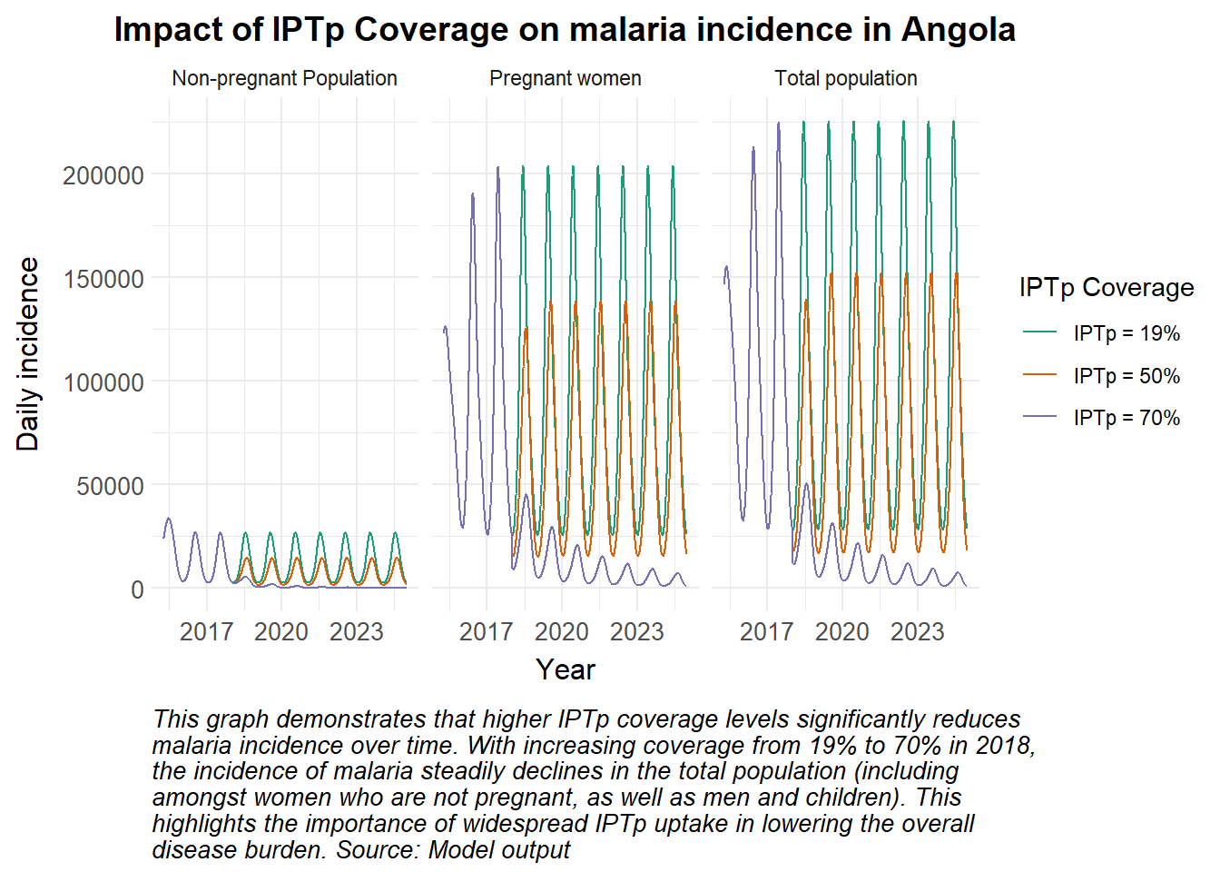
# IPTp coverage scenarios
# Baseline (19%), 50%, 70% IPTp coverage
iptp_scenarios <- c(0.19, 0.5, 0.7) 

# Run the model for each IPTp scenario and store the results
results <- lapply(iptp_scenarios, function(iptp_value) {
  parms["iptp"] <- iptp_value
  run_model(times, start, iptpmodel, parms, scenario = paste0("IPTp = ", iptp_value * 100, "%"))
})

# Combine results for all scenarios
results_combined <- bind_rows(results)

Implications for transmission and incidence

Intermittent Preventive Treatment in Pregnancy (IPTp) reduces the number of infections in pregnant women, who are an otherwise vulnerable reservoir for malaria parasites. IPTp is often used in conjunction with other interventions such as ITNs, however, in this example we demonstrate the impact of scenarios of increasing IPTp coverage on incidence.

Show the code
# Plot new malaria cases (cases) over time for each IPTp scenario
results_combined %>% 
  filter(variable %in% c("GInc", "PInc", "TInc"), time > 100) %>% 
ggplot() +
  geom_line(aes(x = date, y = value, color = scenario)) +
  facet_wrap(~variable, labeller = labeller(variable = c(GInc = "Non-pregnant Population", 
                                                           PInc = "Pregnant women", 
                                                           TInc = "Total population"))) +
  scale_colour_manual_health_radar() +
  theme_health_radar() +
  scale_x_date(date_breaks = "3 years", date_labels = "%Y") +
  labs(title = "Impact of IPTp Coverage on malaria incidence in Angola",
    x = "Year", 
    y = "Daily incidence", 
    caption = str_wrap("This graph demonstrates that higher IPTp coverage levels significantly reduces malaria incidence over time. With increasing coverage from 19% to 70% in 2018, the incidence of malaria steadily declines in the total population (including amongst women who are not pregnant, as well as men and children). This highlights the importance of widespread IPTp uptake in lowering the overall disease burden.  Source: Model output"),
    color = "IPTp Coverage")

Back to top