Climate Data Store

About the data portal

The Climate Data Store (CDS), is a comprehensive and open access platform operated by European Centre for Medium-Range Forecasting (ECMWF) for the Copernicus Climate Change Service (C3S).

CDS is a Climate Data Repository providing access to a wide range of datasets including Observations (satellite and in-situ), Climate Reanalyses, Seasonal Forecasts, Climate Projections and Climate Indices. For each dataset, CDS provides an overview, download and documentation pages.

The site provides Training material to facilitate the use of datasets on the CDS. These include practical data processing workflows based on Jupyter notebooks; e-learning modules on key concepts behind the climate data types as well as learning resources from training events.

The site uses, and provides access to, earthkit which is a new open-source Python project developed by ECMWF that offers robust tools to accelerate workflows in weather and climate science. It streamlines data access, processing, analysis and visualization. At the time of publishing, earthkit is still in the BETA stage of development.

The CDS hosts a number of Applications which allow users to explore and visualize the historic, present and future climate.

Accessing the data portal

The Climate Data Store can be accessed via the following url - https://climate.copernicus.eu/climate-data-store

Climate Data Store landing page. Source: Screenshot from https://climate.copernicus.eu/climate-data-store, accessed 30 May 2025.

Users need to register or login to access many of the features on the climate Data Store (the login tab is found in the top right corner of the page). The CDS utilizes ECMWF user account which enables users to access the CDS as well as other ECMWF resources, events and courses. On CDS the user credentials are primarily used to track user activity, manage data access and ensure compliance with data licenses.

Access to the datasets is provided both interactively (manually over the web) or programmatically through an API service. The CDS provides an extensive User guide section which includes; CDS Documentation which provides users with a deeper understanding of what the Climate Data Store is and how best to use it; guidance on how to download data interactively via the CDS website and also how to get data programmatically via an API service.

What datasets are available

The CDS provides a catalogue which lists available datasets. Users can filter this extensive list of datasets through faceted or text-based searches. The site hosts a number of European-focused datasets, so it’s helpful to filter by Spatial coverage to identify those datasets with Global coverage as these would include the southern Africa domain.

Climate Data Store dataset catalogue filtered by global spatial coverage. Source: Screenshot from https://cds.climate.copernicus.eu/datasets?kw=Spatial+coverage%3A+Global, accessed 30 May 2025.

The datasets can also be filtered by Product type. The definitions of the types is provided below since they may not be easily understandable to a non-climate audience

Climate indices: Quantitative measures derived from climate variables (e.g., temperature, precipitation) that capture key aspects of climate variability and change. Examples include the El Niño-Southern Oscillation (ENSO) index and the Standardized Precipitation Index (SPI).
Climate projections: Simulated future climate conditions based on climate models that use different greenhouse gas emission scenarios. These projections provide insights into potential long-term changes in climate but are subject to uncertainties related to model assumptions and future human activities.
Derived reanalysis: Climate datasets produced by applying additional calculations or transformations to primary reanalysis data. These may include indices, bias-corrected fields, or interpolated datasets that enhance usability for specific applications.
In-situ observations: Climate data collected directly at a specific location using ground-based instruments, such as weather stations, buoys, and radiosondes. These measurements provide high-accuracy climate information but have limited spatial coverage.
Reanalysis: A comprehensive dataset generated by combining historical climate observations with numerical weather models to reconstruct past climate conditions. Reanalysis datasets provide globally consistent and gridded climate information, widely used in climate research.
Satellite observations: Climate data collected by remote sensing instruments aboard satellites, covering various atmospheric, oceanic, and land-surface parameters. These observations provide global coverage and long-term records of climate variables such as temperature, precipitation, and sea surface height.
Seasonal forecasts: Predictions of climate conditions (e.g., temperature, precipitation) for upcoming months to a year, based on climate models and historical data. These forecasts help anticipate climate variations such as droughts, monsoons, and extreme weather events.

Some key datasets that may be of interest are:

Satellite observations

Precipitation monthly and daily gridded data from 1979 to present derived from satellite measurements The Global Precipitation Climatology Project (GPCP) provides global estimates of precipitation as monthly means and daily means, based on estimates using microwave and infrared satellite imagery. The dataset utilizes advanced data processing and calibration techniques to ensure accuracy and constancy of data.

Reanalysis

ERA5 hourly data on single levels from 1940 to present The ERA5 reanalysis outputs are grouped into datasets or catalogue entries. This dataset includes key variables of importance to the malaria modelling community including precipitation, near surface air temperatures and winds (and variables which can be used to calculate relative humidity). The spatial resolution is relatively course (0.25°), but it provides data at very high temporal resolution (hourly) and the dataset is updated daily with just a 5 day latency.
ERA5-Land hourly from 1950 to present ERA5-Land is a enhanced spatial resolution version of ERA5 providing data at 9km. It provides a large range of climatic, surface, vegetation and other variables. The dataset is updated daily with just a 5 day latency.

Seasonal forecasts

Seasonal forecast daily and subdaily data on single levels This catalogue provides a multi-system seasonal forecast service. CDS collects, processes and combines the output from several seasonal forecast models and makes them available of user-relevant applications. Forecasts of key variables such as temperature and precipitation are available for retrospective and future seasonal analysis

Climate projections

CMIP6 Climate projections This catalogue provides daily and monthly global climate model projections data from the sixth phase of the Coupled Model Intercomparison Project (CMIP6). A range of variables are provides from a large number of models covering both the historical and future period represented by eight future Shared Socioenomic Pathway (SSP) scenarios.

Key points to consider

Strengths

The Climate Data Store aims to be a one-stop shop for climate data and analysis. It hosts a very large number of key datasets and provides detailed guidance information, training and tools.

Limitations

The CDS is large and can be confusing and intimidating. The focus is on Europe and not southern Africa.

Citing the data portal

Copernicus Climate Data Store (CDS) hosted by the European Centre for Medium-Range Weather Forecast (ECMWF), https://cds.climate.copernicus.eu/

Terms of use

The CDS requires users to register before any content can be downloaded. Datasets or content made available through the site may have different licensing terms which users need to agree to before access to the content is granted.

The full terms of use can be found on the CDS terms of use

How to plot this data?

In this example, we demonstrate how to visualise ERA5 data using the ERA Explorer application provided by Climate Data Store (CDS). The ERA Explorer application allows users to explore the historical climate for anywhere on earth using the ERA5 reanalysis dataset and focuses on four key variables, temperature, rainfall, wind and humidity, all of which are important for Malaria modelling. In the below example we will focus on two different locations in southern Africa.

Users can select a location of interest by clicking on the global interactive map. The application then calculates a set of climate statistics for the selected grid cell (0.25° x 0.25° resolution), which are displayed as a series of plots. These plots can be downloaded as PNG images, and the underlying data can be downloaded in CSV format. The site also links to example Python notebooks to help users understand, replicate, or customize the code.

Note: The data represents average conditions for the entire grid cell, not the precise local environment.

A guidance section, accessible via the “?” icon, provides information on how to use the app; the organisation, the ERA5 dataset and about the data, and how to interpret the plots presented in the app.

To illustrate, two locations in southern Africa with contrasting climates were selected (Fig. 3):

Kariba, Zimbabwe
Mbabane, Eswatini

Fig. 3: ERA Explorer showing the two selected locations

The ERA Explorer provides several types of visualisations which include:

Monthly climatologies (temperature, rainfall and relative humidity)
Annual timeseries (temperature and rainfall)
Annual anomalies (temperature)
Daily climatologies (temperature)
Hourly climatologies (wind)

Each plot is generated automatically, with a brief explanation below describing the method used. While most plots look straightforward, some involve complex processing—particularly those showing relative humidity or hourly wind climatologies.

If users wish to generate their own plots, it is recommended to download the data from the application and to refer to the example python notebooks provided.

Monthly Climatologies

Monthly temperature climatology for Kariba (Zimbabwe) and Mbabane (Eswatini) for the period 1991-2020. We can see Kariba is consistently warmer than Mbabane throughout the year. Kariba’s temperatures peak in spring (Sept–Nov), while Mbabane experiences its warmest temperatures in summer (Dec–Feb). Both locations have their coolest periods in winter (Jun–Aug). Source: Copernicus Climate Change Service (C3S). (2025). ERA Explorer [Web application]. Retrieved from https://era-explorer.climate.copernicus.eu/

Monthly precipitation climatology for Kariba (Zimbabwe) and Mbabane (Eswatini) for the period 1991-2020. Both locations experience a distinct wet season from November to March, with Kariba generally receiving more rainfall during the early summer months (Dec–Feb). Kariba has an extended dry season from May to October, while Mbabane tends to receive more consistent rainfall throughout its drier season. Source: Copernicus Climate Change Service (C3S). (2025). ERA Explorer [Web application]. Retrieved from https://era-explorer.climate.copernicus.eu/

Monthly precipitation climatology for Kariba (Zimbabwe) and Mbabane (Eswatini) for the period 1991-2020. Mbabane generally exhibits higher relative humidity than Kariba throughout the year. While both locations experience lower humidity during the dry season, Kariba shows a more pronounced drop during the hot, dry months of early spring (Sept–Oct), whereas Mbabane’s lowest levels occur during the cooler winter months (Jun–Aug).Source: Copernicus Climate Change Service (C3S). (2025). ERA Explorer [Web application]. Retrieved from https://era-explorer.climate.copernicus.eu/

Annual Timeseries

Annual average temperature for Kariba (Zimbabwe) and Mbabane (Eswatini) for the period 1940-2024. Kariba is consistently around 8°C warmer than Mbabane. A clear warming trend is evident in both locations. Source: Copernicus Climate Change Service (C3S). (2025). ERA Explorer [Web application]. Retrieved from https://era-explorer.climate.copernicus.eu/

Annual total precipitation for Kariba (Zimbabwe) and Mbabane (Eswatini) for the period 1940-2024. Mbabane consistently receives more annual rainfall than Kariba, with both locations showing high interannual variability. Source: Copernicus Climate Change Service (C3S). (2025). ERA Explorer [Web application]. Retrieved from https://era-explorer.climate.copernicus.eu/

Daily Climatologies

Daily temperature climatology for Kariba (Zimbabwe) for the period 1991-2020. There are distinct cool and warm periods throughout the year. The hottest days and nights occur in late October to early November, while the coldest are observed in early July. Source: Copernicus Climate Change Service (C3S). (2025). ERA Explorer [Web application]. Retrieved from https://era-explorer.climate.copernicus.eu/

Daily temperature climatology for Mbabane (Eswatini) for the period 1991-2020. The coldest days and nights occur in early July, while the warmest temperatures are more broadly distributed across the summer months (Dec–Feb), rather than peaking in a single period. Source: Copernicus Climate Change Service (C3S). (2025). ERA Explorer [Web application]. Retrieved from https://era-explorer.climate.copernicus.eu/

Hourly Climatologies

Hourly climatological wind rose for Kariba (Zimbabwe) for the period 1991-2020. Wind direction is highly unidirectional with very little variation, indicating a dominant prevailing wind. The wind speed does vary, suggesting changes in intensity even though the direction remains relatively consistent. Source: Copernicus Climate Change Service (C3S). (2025). ERA Explorer [Web application]. Retrieved from https://era-explorer.climate.copernicus.eu/

Hourly climatological wind rose for Mbabane (Eswatini) for the period 1991-2020. The wind rose indicates that winds come from multiple directions, with a few directions (Westly, West Noth-Westly and South-Eastly) more common than others. This suggests a moderately variable wind regime without a single dominant direction. Wind speeds also show a wide range of variability. Source: Copernicus Climate Change Service (C3S). (2025). ERA Explorer [Web application]. Retrieved from https://era-explorer.climate.copernicus.eu/

Annual Anomalies

Climate warming stripes (annual temperature anomalies relative to the 1961–2010 reference period) for Kariba (Zimbabwe) and Mbabane (Eswatini) for 1940–2024. A clear concentration of red shades in recent decades highlights a warming trend at both locations. Source: Copernicus Climate Change Service (C3S). (2025). ERA Explorer [Web application]. Retrieved from https://era-explorer.climate.copernicus.eu/

How can this data be used in disease modelling?

Using a country-wide, gridded reanalysis product like the Copernicus Climate Data Store (CDS) ERA5 dataset transforms national disease modeling by providing continuous, gap-free environmental drivers across the entirety country. Unlike scattered point-source station observations, reanalysis data blends satellite and in-situ observations into numerical weather models, offering a complete historical archive of multi-variable climate fields at a national scale.

To explicitly integrate these environmental conditions into a mathematical model, we expand the mechanistic equations adapted from Mordecai et al. (2013) and Agusto (2020) by utilising a spatially distributed ensemble framework. Rather than calculating a simplified, single national average of weather parameters which commits an ecological fallacy due to the highly non-linear curves governing vector biology we resolve the temperature-dependent human biting rates (a), parasite development rates (gamma_m), daily oviposition rates (ovi), and humidity-driven desiccation mortality (mu_m) at the individual grid-cell level before evaluating the national ordinary differential equation (ODE) system. This ensures that localised climate extremes, such as dry Harmattan dust lanes in the north or humid coastal monsoons in the south, are biologically preserved rather than mathematically smoothed away.

Preparing the data

Using the national hourly ERA5 single-levels dataset, we pull t2m (temperature in Kelvin), d2m (dewpoint in Kelvin), and tp (total precipitation in meters). We converted the thermodynamic metrics into Celsius and compute relative humidity via the Magnus-Tetens formula to map country-wide transmission vectors over time. The key modelling shift here is that we apply the non-linear biological trait equations to each grid cell prior to national summation, yielding an ecologically accurate set of daily forcing arrays.

There are different approaches to explicitly include environmental conditions into an infectious disease model. Specifically, the example below describes temperature-dependent human biting rates, mosquito mortality, and the parasite’s Extrinsic Incubation Period (EIP). It also includes a rainfall-dependent environmental carrying capacity that accounts for hydrological extremes, specifically the physical disruption or “flushing” of aquatic larval habitats during heavy rainfall events exceeding 30 mm.

Show the code

# Load and process the gridded CDS ERA5 data
era5_grid_processed <- read_csv("era5_hourly_nigeria.csv") |> 
  mutate(
    DATE = as_date(valid_time),
    temp_C = t2m - 273.15,
    dew_C = d2m - 273.15,
    # Derive Relative Humidity per grid cell via vapor pressures
    sat_vap_press = 0.6108 * exp((17.27 * temp_C) / (237.7 + temp_C)),
    act_vap_press = 0.6108 * exp((17.27 * dew_C) / (237.7 + dew_C)),
    RH = (act_vap_press / sat_vap_press) * 100,
    # Handle any potential NA values in total precipitation before conversion
    tp_clean = ifelse(is.na(tp), 0, tp),
    PRCP_mm = tp_clean * 1000
  ) |> 
  # Step 2: Apply non-linear biological equations AT THE LOCAL GRID LEVEL using vectorized pmax
  mutate(
    cell_a = pmax(-0.00014 * temp_C^2 + 0.027 * temp_C - 0.322, 0.53),
    cell_gamma_m = pmax(0.000112 * temp_C * (temp_C - 15.38) * sqrt(pmax(0, 35 - temp_C)), 0),
    cell_ovi = pmax(-0.153 * temp_C^2 + 8.61 * temp_C - 97.7, 0),
        
    # Combined local thermal limit + relative humidity desiccation stress
    mu_thermal = -log(pmax(-0.000828 * temp_C^2 + 0.0367 * temp_C + 0.522, 0.01)),
    mu_desicc  = ifelse(RH < 55, 0.04 * exp((55 - RH) * 0.07), 0),
    cell_mu_m  = mu_thermal + mu_desicc,
        
    # Local aquatic larval habitat carrying capacity (incorporating local flushing > 30mm)
    cell_K_factor = ifelse(PRCP_mm > 30, PRCP_mm * 0.3, PRCP_mm + 1)
  ) |> 
  # Step 3: Aggregate responses across all coordinates to form coherent national drivers
  group_by(DATE) |> 
  summarise(
    nat_a       = mean(cell_a, na.rm = TRUE),
    nat_gamma_m = mean(cell_gamma_m, na.rm = TRUE),
    nat_ovi     = mean(cell_ovi, na.rm = TRUE),
    nat_mu_m    = mean(cell_mu_m, na.rm = TRUE),
    nat_K_scale = mean(cell_K_factor, na.rm = TRUE),
    # Keep track of raw aggregated metrics for visual verification and tracking
    TAVG        = mean(temp_C, na.rm = TRUE),
    PRCP        = mean(PRCP_mm, na.rm = TRUE), # Fixed: Use mean to avoid multiplying rainfall across grid totals
    RH_AVG      = mean(RH, na.rm = TRUE),
    .groups = "drop"
  ) |> 
  filter(DATE >= ymd("2010-01-01") & DATE <= ymd("2025-08-23")) |> 
  arrange(DATE)

# Plot 1: Temperature Metrics Over Time
ggplot(data = era5_grid_processed) +
  geom_point(
    aes(x = DATE, y = TAVG),
    colour = "#008751", alpha = 0.5, size = 0.8
  ) +
  theme_health_radar() +
  labs(
    title = "Daily National Average Temperature Values in Nigeria \nfrom 2010 to 2025",
    x = "Year",
    y = "Temperature values (Celsius °)",
    caption = str_wrap("Daily temperatures float consistently between 23 and 35 degree celsius, maintaining an ambient environment that keeps parasite replication and extrinsic incubation continuously active throughout the year.")
  ) +
  ylim(0, NA)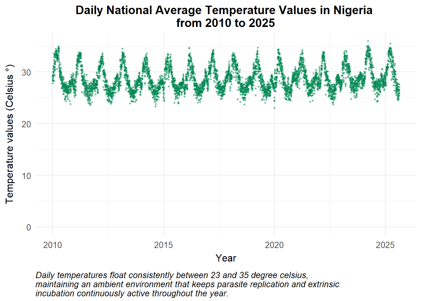

Show the code

# Plot 2: Daily Precipitation (Fixed: calling the correct dataset object)
ggplot(data = era5_grid_processed) +
  geom_point(
    aes(x = DATE, y = PRCP),
    colour = "#1E4D2B", alpha = 0.5, size = 0.8
  ) +
  theme_health_radar() +
  labs(
    title = "Daily Precipitation in Nigeria from 2010 to 2025",
    x = "Year",
    y = "Rainfall values (mm)",
    caption = str_wrap("Daily precipitation averages oscillate predictably between 0 and 6 mm, where regular rainfall expands aquatic breeding capacity, but intense localised storms exceeding 30 mm physically wash away developing larvae.", width = 80)
  ) +
  ylim(0, NA)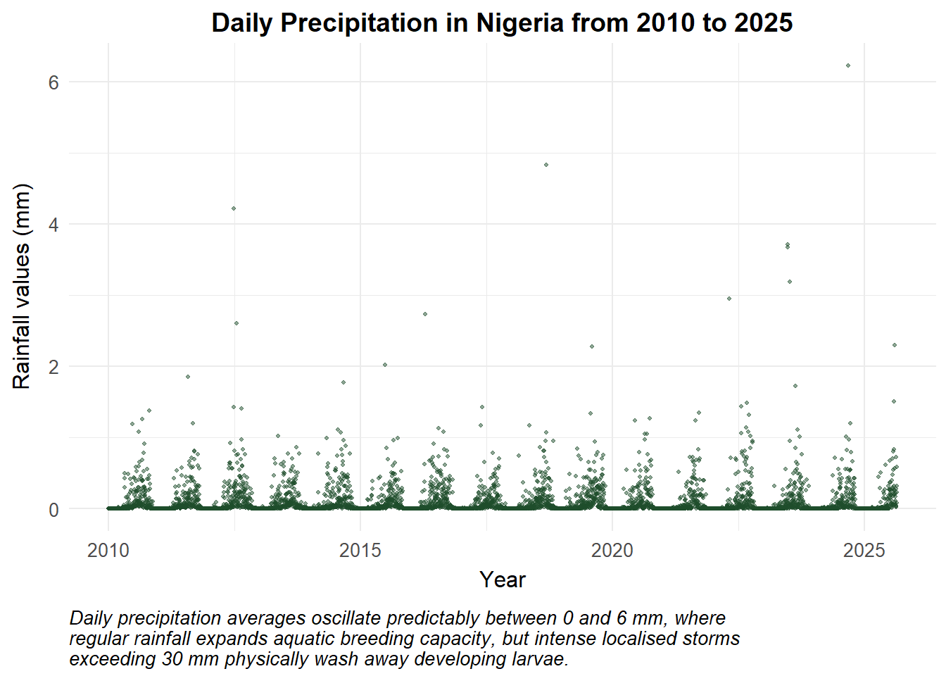

We incorporate pre-resolved, distributed biological parameters directly into our national mathematical model. While other frameworks treat localised metrics as unlinked variables, this model explicitly integrates humidity as a non-linear driver of adult vector desiccation stress within the mortality equation (mu_m).

For this country-wide analysis, we explore national mosquito populations and disease prevalence under the influence of these overlapping environmental forces. We achieve this by holding baseline epidemiological parameters and initial host population structures constant, allowing the shifting, multi-variable climate fields of temperature, precipitation, and relative humidity to dynamically drive transmission potential across the country.

Show the code

# Simulation Timeline Setup
Y = 10
times <- seq(0, 365 * Y, by = 1)

# Extraction of aligned biological forcing arrays
forced_a       <- era5_grid_processed |> fill(nat_a, .direction = "downup") |> pull(nat_a)
forced_gamma_m <- era5_grid_processed |> fill(nat_gamma_m, .direction = "downup") |> pull(nat_gamma_m)
forced_ovi     <- era5_grid_processed |> fill(nat_ovi, .direction = "downup") |> pull(nat_ovi)
forced_mu_m    <- era5_grid_processed |> fill(nat_mu_m, .direction = "downup") |> pull(nat_mu_m)
forced_K_scale <- era5_grid_processed |> fill(nat_K_scale, .direction = "downup") |> pull(nat_K_scale)

# Spatially Corrected SEACR-SEI Model Engine
seacr_era5_ensemble <- function(times, start, parameters, a_vec, gamma_m_vec, ovi_vec, mu_m_vec, K_vec) {
  with(as.list(c(start, parameters)), {
    P = S + E + A + C + R + G
    M = Sm + Em + Im
    
    t_day <- min(floor(times) + 1, length(a_vec))
    
    # Pull pre-resolved biological parameters for day t
    a       <- a_vec[t_day]
    gamma_m <- gamma_m_vec[t_day]
    ovi     <- ovi_vec[t_day]
    mu_m    <- mu_m_vec[t_day]
    K       <- Km * K_vec[t_day]
    
    # Transmission dynamics based on aggregated local suitability
    Infectious <- C + zeta_a * A
    lambda.v   <- a * (M / P) * b * (Im / M)
    lambda.h   <- a * c * (Infectious / P)
    
    # System Differentials
    dSm  <- ovi * (1 - M / K) * M - lambda.h * Sm - mu_m * Sm
    dEm  <- lambda.h * Sm - (gamma_m + mu_m) * Em
    dIm  <- gamma_m * Em - mu_m * Im
    
    dS   <- mu_h * P - lambda.v * S + rho * R - mu_h * S
    dE   <- lambda.v * S - (gamma_h + mu_h) * E
    dA   <- pa * gamma_h * E + pa * gamma_h * G - (delta + mu_h) * A
    dC   <- (1 - pa) * gamma_h * E + (1 - pa) * gamma_h * G - (r + mu_h) * C
    dR   <- delta * A + r * C - (lambda.v + rho + mu_h) * R
    dG   <- lambda.v * R - (gamma_h + mu_h) * G
    dCInc <- lambda.v * (S + R)
    
    list(c(dSm, dEm, dIm, dS, dE, dA, dC, dR, dG, dCInc))
  })
}

# Complete system initialisation
initial_state <- c(Sm = 70000, Em = 25000, Im = 35000, S = 85000, E = 15000, A = 8000, C = 6000, R = 4000, G = 1000, CInc = 0)
parameters    <- c(b = 0.72, c = 0.52, r = 1/21, rho = 1/150, delta = 1/140, zeta_a = 0.4, pa = 0.38, mu_h = 1/(60 * 365), gamma_h = 1/10, Km = 45000)

# Run the spatially corrected system
out_Nigeria <- ode(y = initial_state, times = times, func = seacr_era5_ensemble, parms = parameters,
 a_vec = forced_a, gamma_m_vec = forced_gamma_m, ovi_vec = forced_ovi, mu_m_vec = forced_mu_m, K_vec = forced_K_scale)

df_nigeria_results <- as_tibble(as.data.frame(out_Nigeria)) |> 
  mutate(P = S + E + A + C + R + G,
         M = Sm + Em + Im,
         Inc = c(0, diff(CInc)),
         date = ymd("2010-01-01") + time, 
         Country = "Nigeria"
  ) |>
  pivot_longer(cols = c(-time, -date, -Country), names_to = "variable", values_to = "value")

Changes in vector population

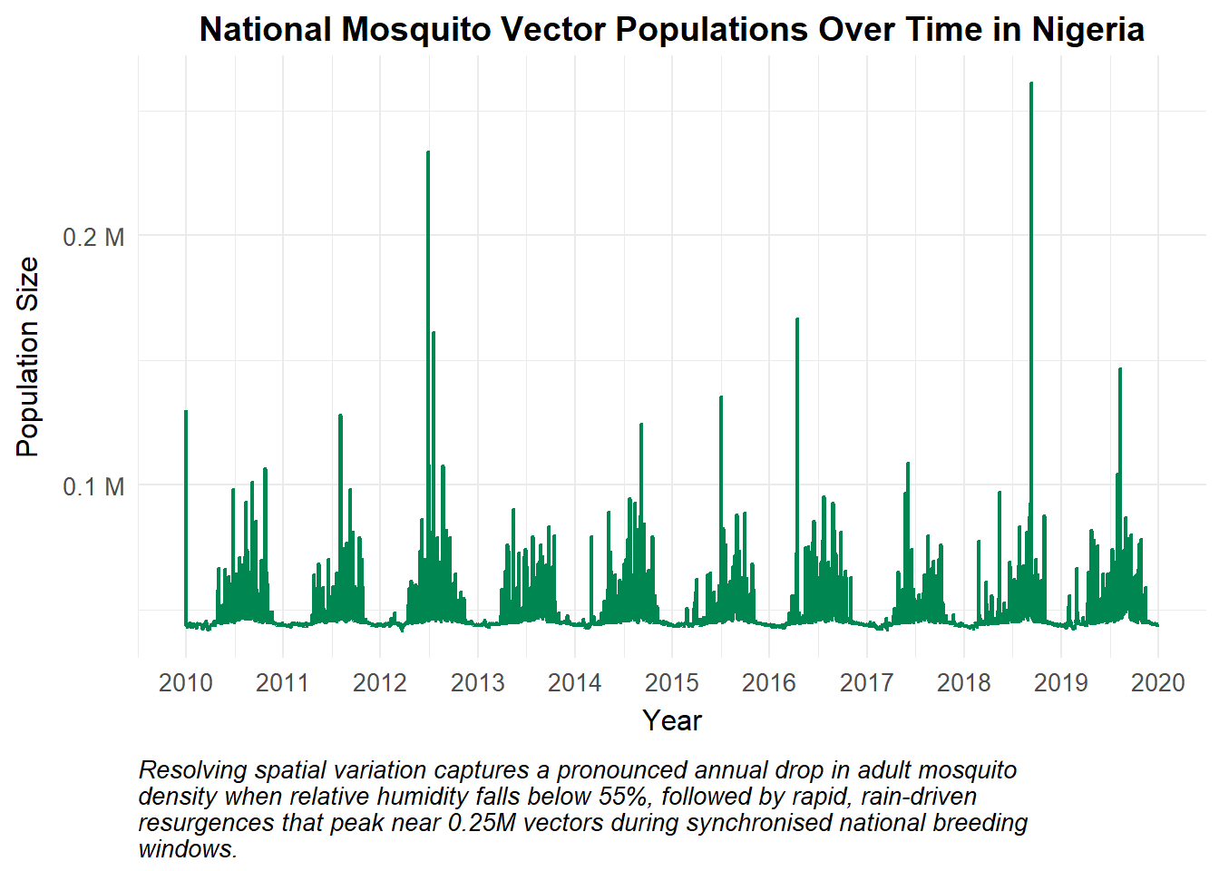
The interactions between local environmental stressors create distinct macro-trends in the mosquito population (M). During the dry season, low relative humidity values driven by the regional Harmattan wind patterns induce heavy desiccation stress across northern grids, spiking vector mortality (mu_m) and causing a substantial drop in the overall national vector population. When the seasonal monsoon rains arrive, this atmospheric pressure eases and expanding aquatic breeding habitats across all grid coordinates trigger a rapid, widespread resurgence in mosquito populations across the country.

Show the code

df_nigeria_results |> 
  filter(variable == "M") |> 
  ggplot() +
  geom_line(aes(x = date, y = value), colour = "#008751", size = 0.8) +
  theme_health_radar() +
  scale_y_continuous(labels = scales::label_number(suffix = " M", scale = 1e-6)) +
  scale_x_date(date_breaks = "1 year", date_labels = "%Y") +
  labs(
    title = "National Mosquito Vector Populations Over Time in Nigeria", 
    x = "Year", y = "Population Size",
    caption = str_wrap("Resolving spatial variation captures a pronounced annual drop in adult mosquito density when relative humidity falls below 55%, followed by rapid, rain-driven resurgences that peak near 0.25M vectors during synchronised national breeding windows.")
  )

Implications for transmission

By processing climate fields on a distributed mesh, our model explicitly capture transmission bottlenecks that simple aggregated models tend to miss.

The resulting simulation demonstrates an intense, perennial transmission profile that is bounded by seasonal transitions. During dry-season intervals, transmission slows considerably; even though ambient temperatures remain high enough to support rapid parasite development (EIP), the low relative humidity shortens adult mosquito lifespans, meaning few vectors survive long enough to become fully infectious (Im). Once the wet season breaks, the pairing of optimal temperatures and elevated relative humidity extends vector longevity, unleashing high-velocity transmission cycles that produce distinct, broad annual waves in clinical cases (C) across the population.

Note that these outputs represent illustrative indicators of transmission potential derived from multi-variable environmental suitability. In operational contexts, recorded clinical case data may deviate from these metrics due to healthcare access limits, localised interventions, or diagnostic availability.

Show the code

df_nigeria_results |> 
  filter(variable == "C", time > 100) |>
  ggplot()+
  geom_line(aes(x = date, y = value), colour = "#008751", size = 0.8) +
  theme_health_radar() +
  scale_x_date(date_breaks = "1 year", date_labels = "%Y") +
  labs(
    title = "Daily Symptomatic Cases Values in the Nigerian Human Population", 
    x = "Year", y = "Number of Cases",
    caption = str_wrap("The transmission profile displays highly responsive, clockwork seasonality where a distinct annual dry-season drop down to 2,500 cases is followed by a sharp monsoonal surge peaking near 20,000 cases as environmental conditions recover.", width = 150)
  ) +
  ylim(0, NA)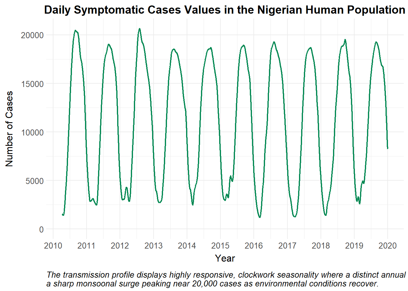

Policy implications

Models that evaluate non-linear temperature, rainfall, and relative humidity matrices on a distributed grid enable the National Malaria Elimination Programme (NMEP) of a country to transition from reactive management to proactive, forecast-driven public health planning:

Because this framework captures how relative humidity acts as a key survival bottleneck for vectors, control programs can time the distribution of Long-Lasting Insecticidal Nets (LLINs) and seasonal chemoprevention to conclude right before the national humidity upswing, targeting the vector population at its most vulnerable point. Also th Rapid Diagnostic Tests (RDTs) and Artemisin-based Combination Therapies (ACTs) can be moved into regional distribution hubs ahead of the surge, preventing stockouts during high-transmission months.

Incorporating continuous Copernicus Climate Data Store feeds helps health authorities identify anomalous years such as prolonged rainy seasons or unseasonably humid dry intervals allowing teams to adjust national control budgets and operational timelines dynamically.

Citations

Agusto F. B., Gumel A. B., & Parham P. E. Qualitative assessment of the role of temperature variations on malaria transmission dynamics. Journal of Biological Systems, 23(04), 1550030 (2015). https://doi.org/10.1142/S0218339015500308
Copernicus Climate Change Service (C3S). ERA5 hourly data on single levels from 1940 to present. Copernicus Climate Data Store (CDS). Nigeria domain reanalysis data asset accessed May 2025. https://cds.climate.copernicus.eu/
Mordecai EA, Paaijmans KP, Johnson LR, Balzer C, Ben-Horin T, de Moor E, McNally A, Pawar S, Ryan SJ, Smith TC, Lafferty KD. Optimal temperature for malaria transmission is dramatically lower than previously predicted. Ecol Lett. 2013 Jan;16(1):22-30. https://pubmed.ncbi.nlm.nih.gov/23050931/
Paaijmans KP, Wandago MO, Githeko AK, Takken W. Unexpected high losses of Anopheles gambiae larvae due to rainfall. PLoS One. 2007 Nov 7;2(11):e1146. https://doi.org/10.1371/journal.pone.0001146
Suh, E., Stopard, I.J., Lambert, B. et al. Estimating the effects of temperature on transmission of the human malaria parasite, Plasmodium falciparum. Nature Communications 15, 3230 (2024). https://doi.org/10.1038/s41467-024-47265-w
Traoré B., Sangaré B., Traoré S. A mathematical model of malaria transmission with structured vector population and seasonality. Journal of Applied Mathematics, 1, 6754097 (2017). https://doi.org/10.1155/2017/6754097 https://doi.org/10.4269/ajtmh.2005.73.1072