The CRU TS (Climatic Research Unit gridded Time Series) dataset is a global, high-resolution, land-based climate dataset that provides monthly records on a 0.5° grid (approximately 55.5 km by 55.5 km at the equator, varying slightly by latitude). The dataset is derived by the interpolation of monthly climate anomalies from extensive networks of weather station observations, offering data from 1901 onwards. This observational dataset consists of ten observed and derived climate variables, such as temperature and precipitation (see Variables list below), making it useful for many types of users, in diverse research areas and applications and has been widely adopted in research and policy work.
Updated annually, the dataset follows a versioning system, CRU TS vX.YY. Where ‘X’ reflects major updates in methodology and ‘YY’ indicates minor refinements, extending its temporal coverage and improving data quality, compared to previous versions.
For more information regarding all CRU datasets see CRU-data
Users can also find more information about the CRU dataset here:
The Climatic Research Unit (CRU) at the University of East Anglia is the creator of this dataset. Users can download it directly from their website, which lists all available datasets, with the most recent version listed at the top. When downloading from CRU, the file provided are for the full global dataset and are available in both ASCII and NetCDF formats. This is the best source for accessing the latest version of the data.
Version
Variables
Resolution
Spatial Extent
File Format
Latest available
cld, dtr, frs, pet, pre, tmp, tmn, tmx, vap, wet
0.5° (~55.5km x ~55.5km)
Global
netCDF (.nc), ASCII (.dat)
The Climate Data Store also provides a version of the CRU dataset for users to download. It can be accessed here. However, the version available on the Climate Data Store is not always the most up-to-date. The data is provided in NetCDF format.
Version
Variables
Resolution
Spatial Extent
File Format
May not be the latest
pre, tmp, tmn, tmx
0.5° (~55.5km x ~55.5km), 1.0° (~111km x ~111km), 2.5° (~277.5km x ~277.5km)
Global
netCDF (.nc)
The KNMI Climate Explorer is another platform where users can download CRU data. The dataset can be specified on their Monthly Observations page, where the latest version of CRU is usually available. Users can download data for a specific grid point or area or create a custom subset using a mask (e.g., a shapefile). Data provided in NetCDF format.
Version
Variables
Resolution
Spatial Extent
File Format
Typically up-to-date
cld, dtr, frs, pet, pre, tmp, tmn, tmx, vap
0.5° (~55.5km x ~55.5km), 1.0° (~111km x ~111km), 2.5° (~277.5km x ~277.5km)
User specified
netCDF (.nc)
What the data looks likes
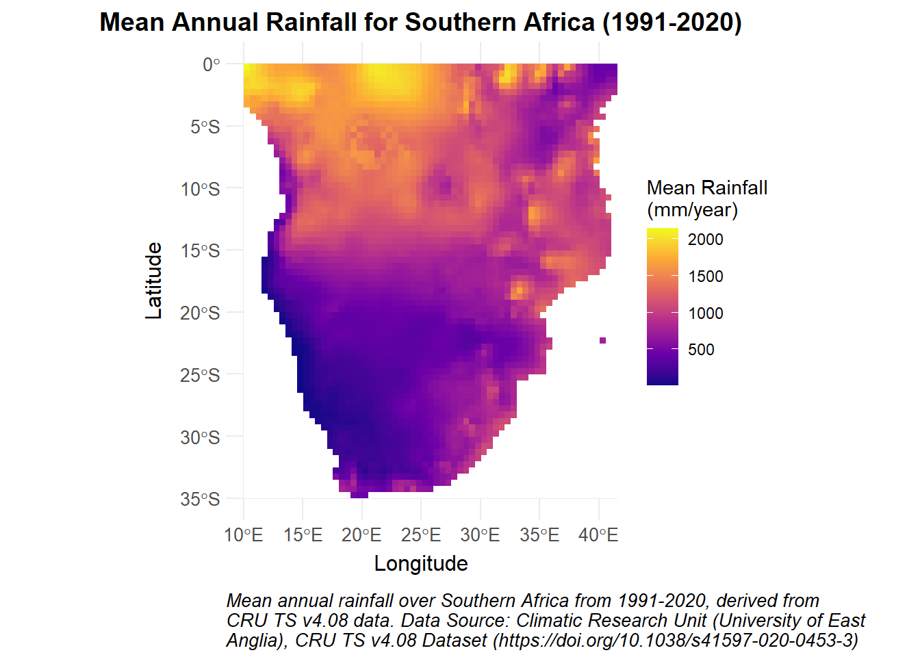
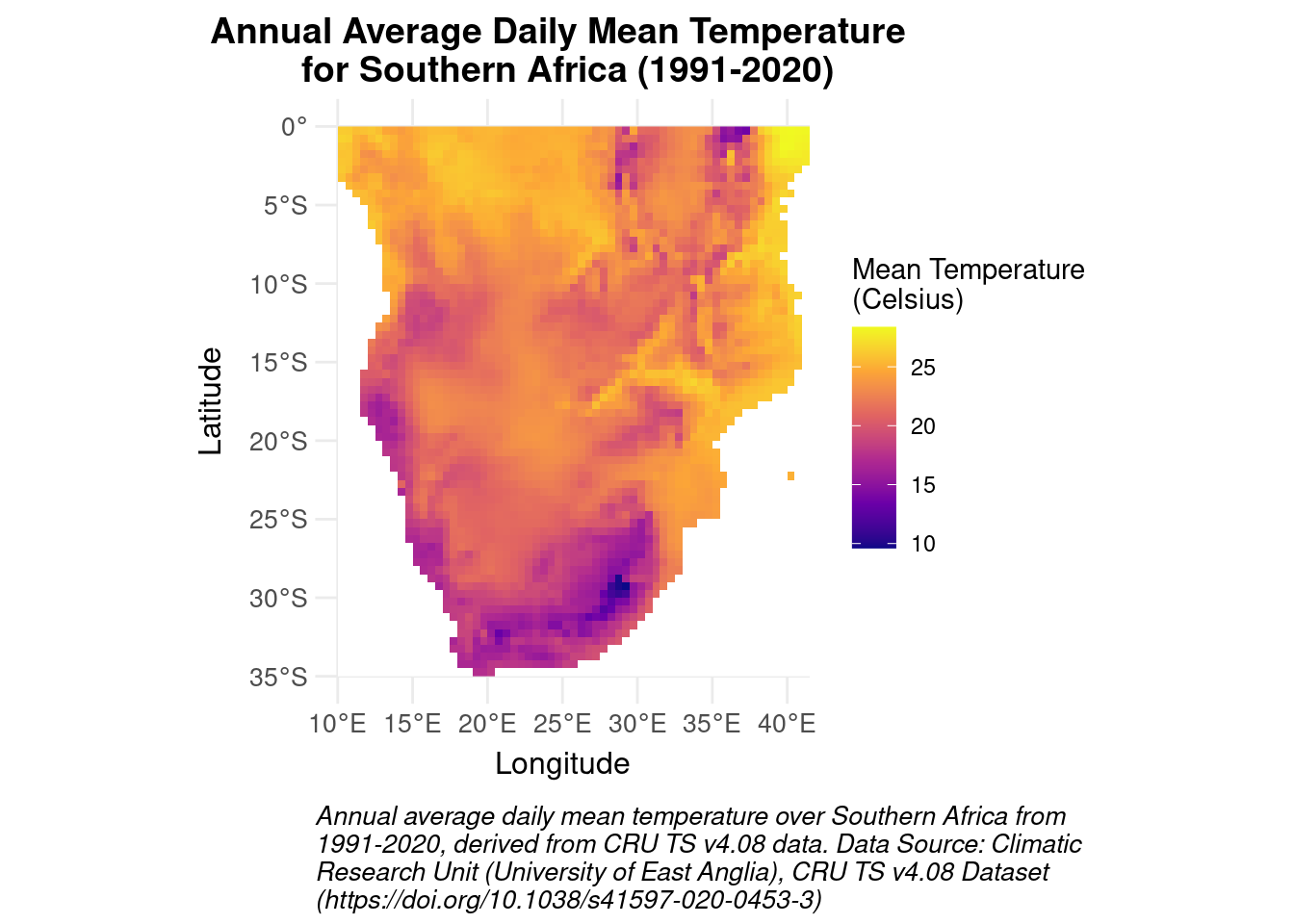
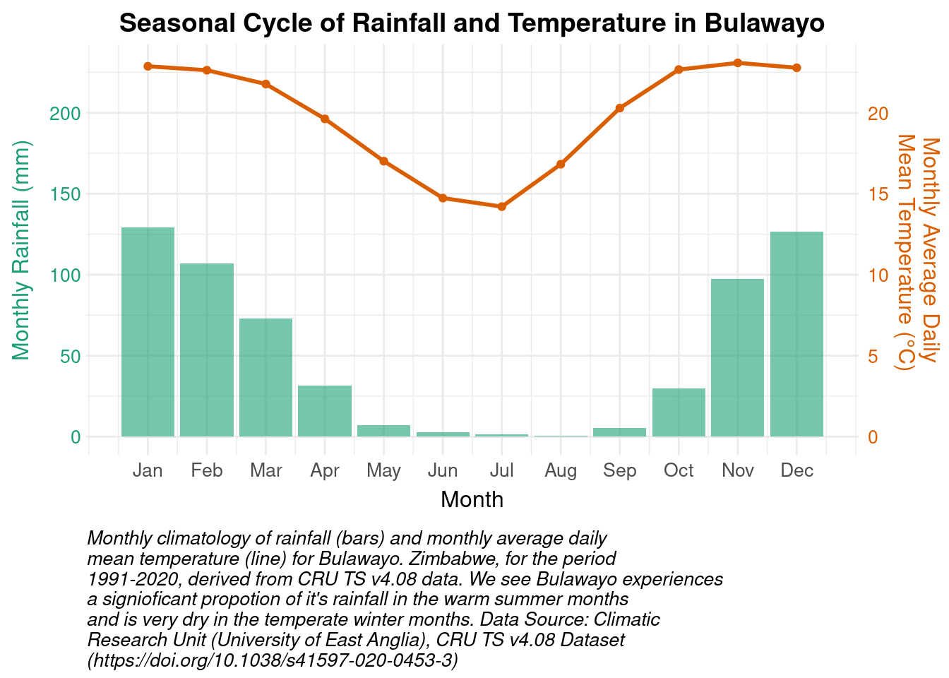
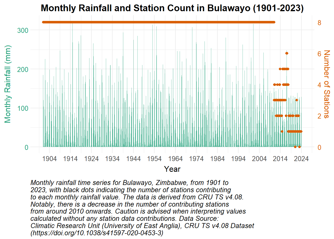
Below are a few plots to give a better sense of what the CRU dataset looks like. The first two are spatial plots over Southern Africa, illustrating the spatial resolution and the coarseness of the 0.5° × 0.5° grid. The final three plots focus on a single grid cell and show the seasonal cycle and time series data for that location.
Spatial plots of key variables
Show the code
library(terra)library(ggplot2)library(tidyterra) library(stringr)# Read the NetCDF file using terrafig1_mean_annual_rainfall <-rast("data/Fig1_MeanAnnualRainfall_CRU_TS-4.08_1991-2020_SouthernAfrica.nc")# Make 0 values NAfig1_mean_annual_rainfall[fig1_mean_annual_rainfall ==0] <-NA# Create the plotggplot() +geom_spatraster(data = fig1_mean_annual_rainfall,na.rm =TRUE ) +scale_fill_continuous_health_radar(option ="plasma", na.value ="white",name ="Mean Rainfall\n(mm/year)"# Removed trailing comma ) +coord_sf(xlim =c(10, 40),ylim =c(-35, 0) ) +theme_health_radar() +labs(title ="Mean Annual Rainfall for Southern Africa (1991-2020)",x ="Longitude", y ="Latitude",caption =str_wrap("Mean annual rainfall over Southern Africa from 1991-2020, derived from CRU TS v4.08 data. Data Source: Climatic Research Unit (University of East Anglia), CRU TS v4.08 Dataset (https://doi.org/10.1038/s41597-020-0453-3)", width =75) )
Show the code
fig2_mean_monthly_avg_temperature <-rast("data/Fig2_MeanMonthlyAverageTemp_CRU_TS-4.08_1991-2020_SouthernAfrica.nc")# Create the plotggplot() +geom_spatraster(data = fig2_mean_monthly_avg_temperature,na.rm =TRUE ) +scale_fill_continuous_health_radar(option ="plasma", na.value ="white",name ="Mean Temperature\n(Celsius)"# Removed trailing comma ) +coord_sf(xlim =c(10, 40),ylim =c(-35, 0) ) +theme_health_radar() +labs(title ="Annual Average Daily Mean Temperature \n for Southern Africa (1991-2020)",x ="Longitude", y ="Latitude",caption =str_wrap("Annual average daily mean temperature over Southern Africa from 1991-2020, derived from CRU TS v4.08 data. Data Source: Climatic Research Unit (University of East Anglia), CRU TS v4.08 Dataset (https://doi.org/10.1038/s41597-020-0453-3)", width =75) )
Show the code
library(readr)fig3_PRCPTOT_mon <-read_csv("data/Fig3_PRCPTOT_mon_CRU_TS-4.08_199101-202012_climatology_Bulawayo.csv")fig3_tas_mon <-read_csv("data/Fig3_tas_mon_CRU_TS-4.08_199101-202012_climatology_Bulawayo.csv")# Create the climatology plotggplot() +# Rainfall barsgeom_col(data = fig3_PRCPTOT_mon,aes(x = time, y = PRCPTOT, fill ="Rainfall"),alpha =0.6 ) +# Temperature linegeom_line(data = fig3_tas_mon,aes(x = time, y = tas *10, color ="Temperature"),linewidth =1 ) +geom_point(data = fig3_tas_mon,aes(x = time, y = tas *10, color ="Temperature") ) +# Use standardized color scales with explicit valuesscale_fill_manual(values =setNames(theme_health_radar_colours[1], "Rainfall")) +scale_colour_manual(values =setNames(theme_health_radar_colours[2], "Temperature")) +# Primary axis (rainfall)scale_y_continuous(name ="Monthly Rainfall (mm)",sec.axis =sec_axis(~./10, name ="Monthly Average Daily\n Mean Temperature (°C)") ) +scale_x_continuous(breaks =1:12,labels =c("Jan", "Feb", "Mar", "Apr", "May", "Jun", "Jul", "Aug", "Sep", "Oct", "Nov", "Dec") ) +theme_health_radar() +theme(axis.title.y.right =element_text(color = theme_health_radar_colours[2]), # Match temperature line coloraxis.text.y.right =element_text(color = theme_health_radar_colours[2]), # Match temperature line coloraxis.title.y.left =element_text(color = theme_health_radar_colours[1]), # Match rainfall bar coloraxis.text.y.left =element_text(color = theme_health_radar_colours[1]), # Match rainfall bar colorlegend.position ="none" ) +labs(title ="Seasonal Cycle of Rainfall and Temperature in Bulawayo",x ="Month",caption =str_wrap("Monthly climatology of rainfall (bars) and monthly average daily mean temperature (line) for Bulawayo. Zimbabwe, for the period 1991-2020, derived from CRU TS v4.08 data. We see Bulawayo experiences a signioficant propotion of it's rainfall in the warm summer months and is very dry in the temperate winter months. Data Source: Climatic Research Unit (University of East Anglia), CRU TS v4.08 Dataset (https://doi.org/10.1038/s41597-020-0453-3)", width =75) )
Show the code
fig4_PRCPTOT_mon <-read_csv("data/Fig4_PRCPTOT_mon_CRU_TS-4.08_190101-202312_Bulawayo.csv")# Create the timeseries plotggplot() +# Rainfall barsgeom_col(data = fig4_PRCPTOT_mon,aes(x = time, y = PRCPTOT, fill ="Rainfall"),alpha =0.6 ) +# Station count linegeom_point(data = fig4_PRCPTOT_mon,aes(x = time, y = stn *40, color ="Station Count"),linewidth =0.8 ) +# Use standardized color scales with explicit valuesscale_fill_manual(values =setNames(theme_health_radar_colours[1], "Rainfall")) +scale_colour_manual(values =setNames(theme_health_radar_colours[2], "Station Count")) +# Primary axis (rainfall)scale_y_continuous(name ="Monthly Rainfall (mm)",sec.axis =sec_axis(~./40, name ="Number of Stations",breaks =seq(0, 10, 2), # Force breaks from 0 to 10 ) ) +scale_x_date(date_breaks ="10 years",date_labels ="%Y" ) +theme_health_radar() +theme(axis.title.y.right =element_text(color = theme_health_radar_colours[2]),axis.text.y.right =element_text(color = theme_health_radar_colours[2]), axis.title.y.left =element_text(color = theme_health_radar_colours[1]),axis.text.y.left =element_text(color = theme_health_radar_colours[1]), legend.position ="none" ) +labs(title ="Monthly Rainfall and Station Count in Bulawayo (1901-2023)",x ="Year",caption =str_wrap("Monthly rainfall time series for Bulawayo, Zimbabwe, from 1901 to 2023, with black dots indicating the number of stations contributing to each monthly rainfall value. The data is derived from CRU TS v4.08. Notably, there is a decrease in the number of contributing stations from around 2010 onwards. Caution is advised when interpreting values calculated without any station data contributions. Data Source: Climatic Research Unit (University of East Anglia), CRU TS v4.08 Dataset (https://doi.org/10.1038/s41597-020-0453-3)", width =75) )
Show the code
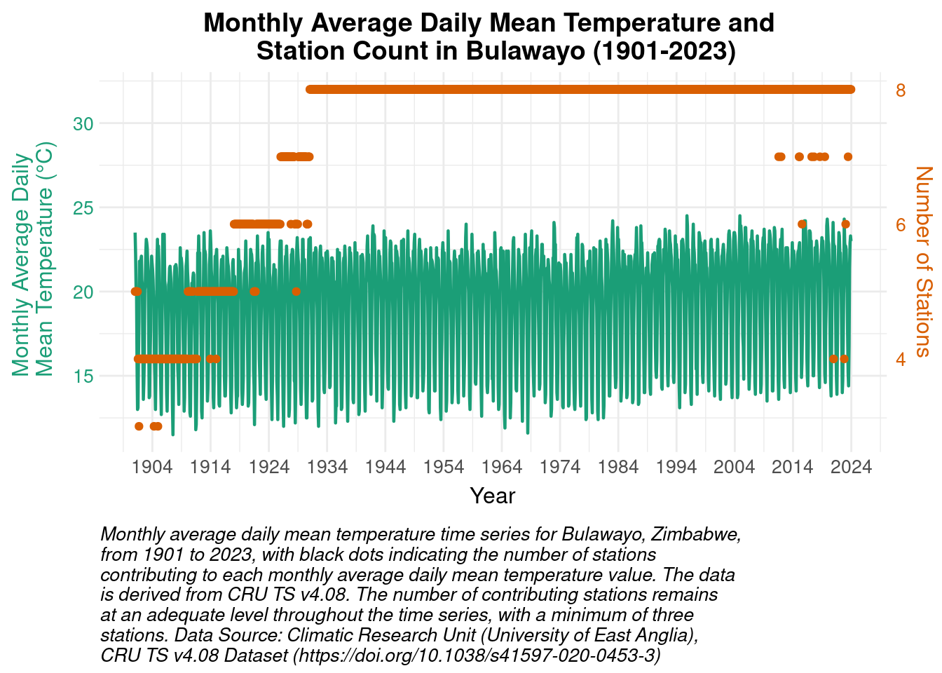
fig5_tas_mon <-read_csv("data/Fig5_tas_mon_CRU_TS-4.08_190101-202312_Bulawayo.csv")# Create the timeseries plotggplot() +# Temperature barsgeom_line(data = fig5_tas_mon,aes(x = time, y = tas -273.15, color ="Temperature"),linewidth =0.8 ) +# Station count linegeom_point(data = fig5_tas_mon,aes(x = time, y = stn *4, color ="Station Count"),linewidth =0.8 ) +# Use standardized color scales with explicit valuesscale_colour_manual(values =c( "Temperature"= theme_health_radar_colours[1], "Station Count"= theme_health_radar_colours[2])) +#scale_fill_manual(values = setNames(theme_health_radar_colours[1], "Temperature")) +#scale_colour_manual(values = setNames(theme_health_radar_colours[2], "Station Count")) +# Primary axis (temperature)scale_y_continuous(name ="Monthly Average Daily \n Mean Temperature (°C)",sec.axis =sec_axis(~./4, name ="Number of Stations",breaks =seq(0, 10, 2), # Force breaks from 0 to 10 ) ) +scale_x_date(date_breaks ="10 years",date_labels ="%Y" ) +theme_health_radar() +theme(axis.title.y.right =element_text(color = theme_health_radar_colours[2]),axis.text.y.right =element_text(color = theme_health_radar_colours[2]), axis.title.y.left =element_text(color = theme_health_radar_colours[1]),axis.text.y.left =element_text(color = theme_health_radar_colours[1]), legend.position ="none" ) +labs(title ="Monthly Average Daily Mean Temperature and \n Station Count in Bulawayo (1901-2023)",x ="Year",caption =str_wrap("Monthly average daily mean temperature time series for Bulawayo, Zimbabwe, from 1901 to 2023, with black dots indicating the number of stations contributing to each monthly average daily mean temperature value. The data is derived from CRU TS v4.08. The number of contributing stations remains at an adequate level throughout the time series, with a minimum of three stations. Data Source: Climatic Research Unit (University of East Anglia), CRU TS v4.08 Dataset (https://doi.org/10.1038/s41597-020-0453-3)", width =75) )
Key points to consider
CRU provides users with the number of stations used to build each datum within the CRU TS dataset. The NetCDF-formatted (CF-1.4 compliant) CRU TS data output files (for all variables except PET) contain two data variables, the named one, (i.e., ‘tmp’), and a station count (‘stn’) giving the number of stations. If working with ASCII text output files, CRU also publishes a separate station count metadata file. The station counts vary between 0 (no cover, climatology inserted, see Interpolation above), and eight (the maximum station count for interpolation). The ‘stn’ data may be used to quantify uncertainty, most particularly by excluding cells with a zero count, as these will have been set to the default climatology ((i.e., long-term average values from a reference period when no observations are available). The station count can vary widely through space and time and per variable, see figures 4 and 5 above.
Strengths
The dataset is widely used and evaluated.
It provides a number of useful variables for malaria modelling.
It provides and long and continuous record.
Limitations
The skill1 of the dataset relies heavily on the density of the station network. The density over southern Africa is very poor with some areas not having any available stations, or they are are very far away in climatically very different regions.
The data is monthly which limits the usefulness of the dataset which may require higher temporal resolution data.
The stations come from a number of different networks and they are not strictly homogenized so caution should be use in any trend analysis.
Citing the data
Harris, I., Osborn, T.J., Jones, P. et al. Version 4 of the CRU TS monthly high-resolution gridded multivariate climate dataset. Sci Data 7, 109 (2020). https://doi.org/10.1038/s41597-020-0453-3
Terms of use
The various datasets on the CRU website are provided for all to use, provided the sources are acknowledged. Acknowledgment should preferably be by citing one or more of the papers referenced. The website can also be acknowledged if deemed necessary.
Select the required variables from the CRU TS dataset (daily maximum and minimum temperature and rainfall).
Generate an area-average spatial subset for the full record period (in this case, for the Mopani District, Limpopo Province, South Africa for the period 1901 - 2023).
Download the resulting data as text files.
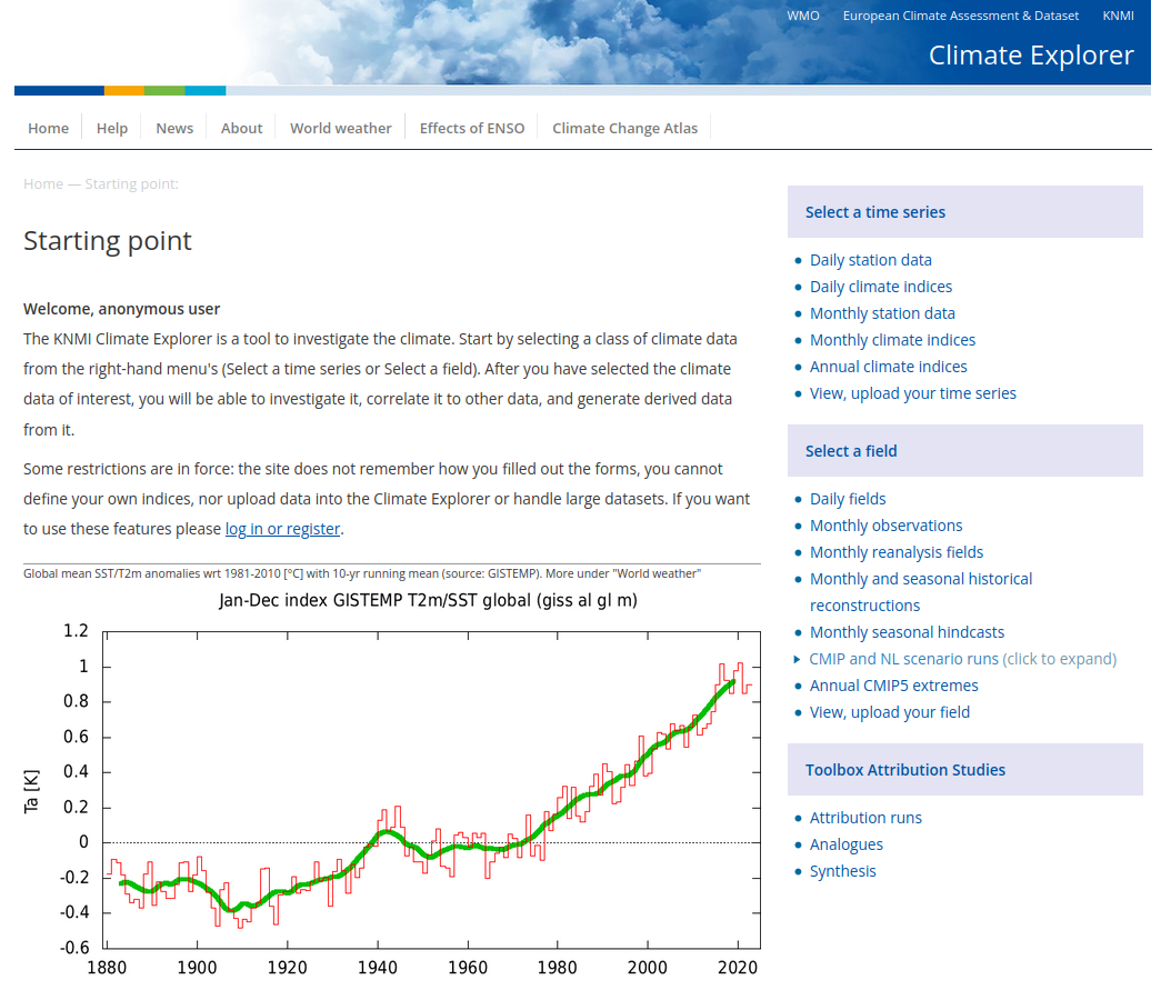
While the KNMI Climate Explorer allows anonymous access, it is recommended to register and login to access more features.
The CRU TS dataset is accessible through the side menu under Select a field > Monthly observations
Fig. 1: KNMI Climate Explorer home page
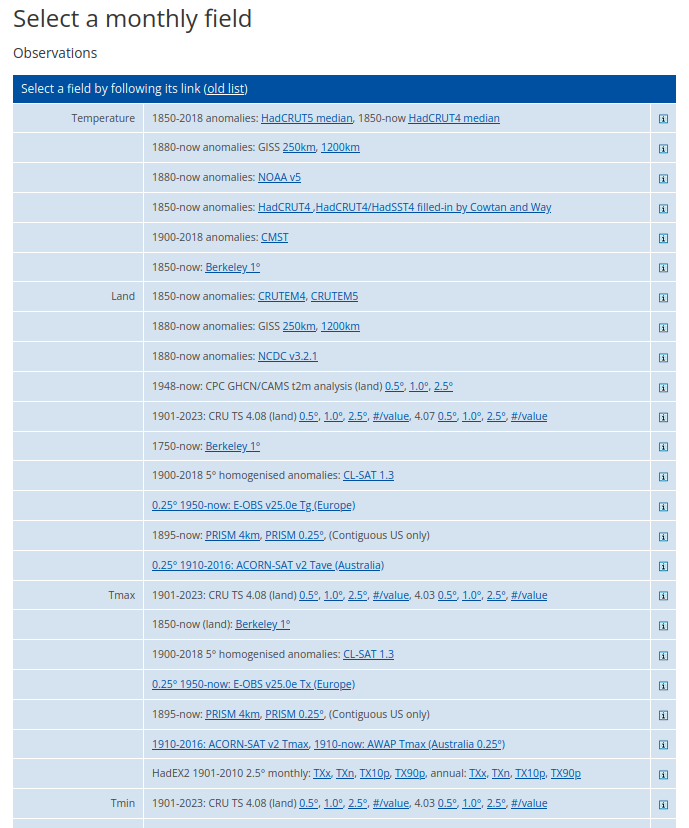
The site lists a number of monthly fields by variable / categories (the names of which may appear somewhat confusing at first). The CRU TS can be found under the different variables and in this visualisation example we will focus on the data listed under the variables Tmax (daily maximum temperature).
Users can select the data at different spatial resolutions (0.5°, 1.0°, 2.5°). A metadata variable #/value is also available, indicating the number of weather stations used to calculate each gridcell’s value, ranging from 0 to 8 stations.
Fig. 2: KNMI Climate Explorer Monthly Observation list of datasets
Regridding to a lower spatial or temporal resolution
Computing of anomalies from a climatological mean, or from zonal mean.
It also provides a link to download the dataset itself (though it recommends that users rather utilise the authoritative site).
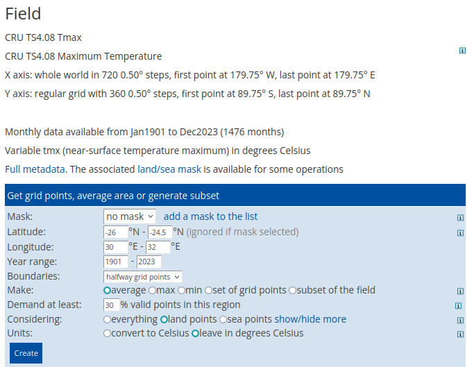
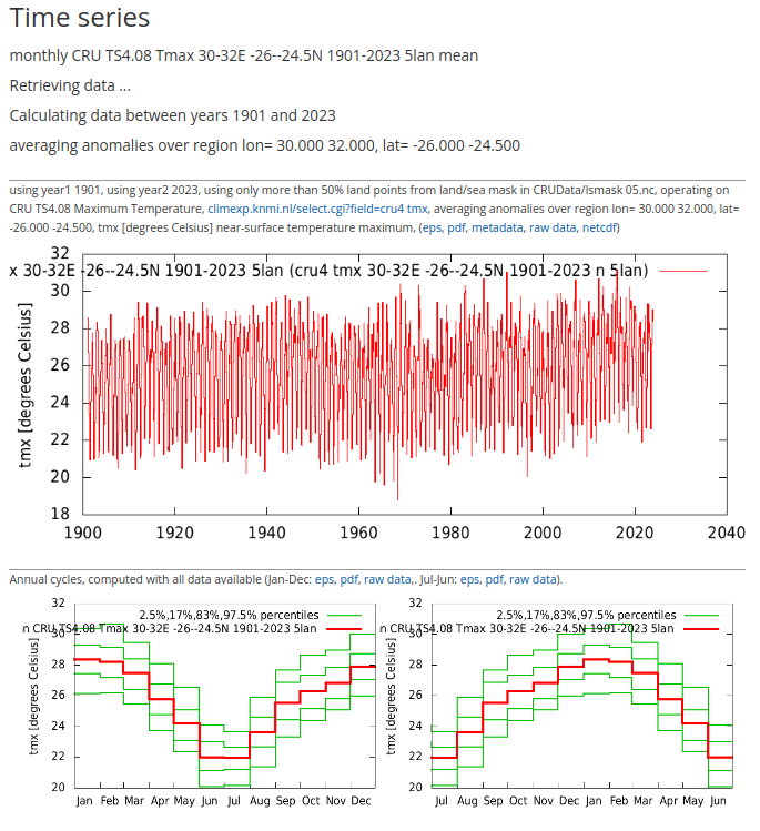
For our purposes, we generate an area average for a spatial subset for the Mopani District, Limpopo Province, South Africa by specifying the latitude and longitude bounds.
Fig. 3: KNMI Climate Explorer tools used to create the spatial subset.
The output includes:
A times series
The annual cycle
Anomalies relative to the annual cycle.
The site generates basic plots of the output, that can be downloaded either in eps or pdf format. The data itself can be downloaded as the raw data (txt format) or as a netcdf file. Both formats include detailed metadata along with the data itself.
Fig. 4: KNMI Climate Explorer time page presenting the time series output.
How to plot this data?
The downloaded time series can be used for various analyses and visualisations.
In this example, we perform a simple sanity check on the data by exploring the variability and trends in the climate over the historical period for the Mopani District. Specifically, we present annual anomalies for daily maximum and daily minimum temperature and rainfall.
Analysis steps
Calculation of annual mean or total values for daily maximum and minimum temperature and rainfall.
We use a July–June year to align with the malaria season, which primarily occurs in summer.
Calculate the average (baseline) climate for the 30-year period 1981-2010.
This is a standard climatological baseline and corresponds with relatively complete station coverage globally.
Compute anomalies by subtracting the baseline from each year’s value.
Include the metadata #/value (station count) as an annual average to provide an indication of the data quality across the record.
Interpretation and discussion
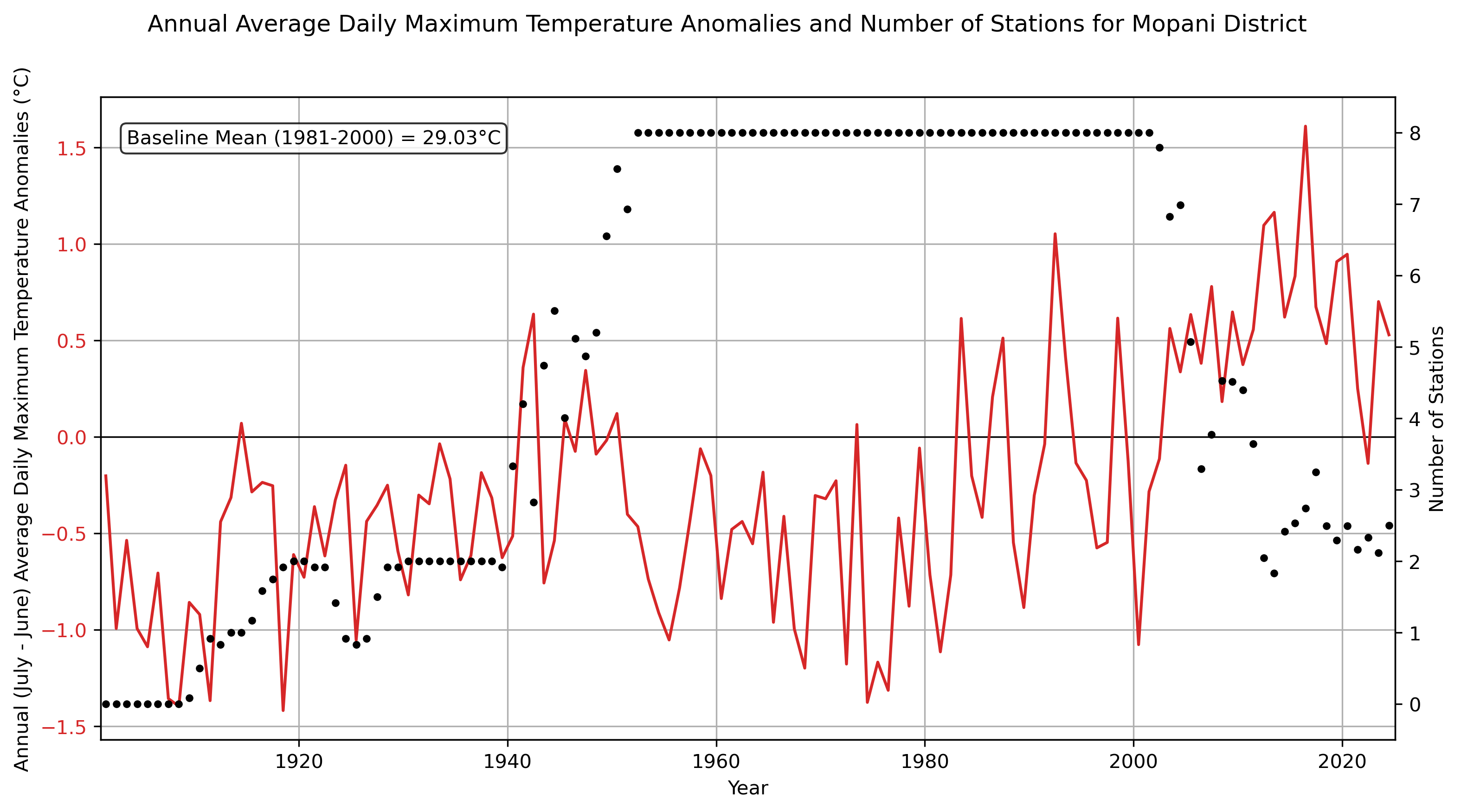
Daily Maximum Temperature (Tmax): The average is 29°C (Fig. 5). The time series shows considerable year-to-year variability and an overall warming trend.
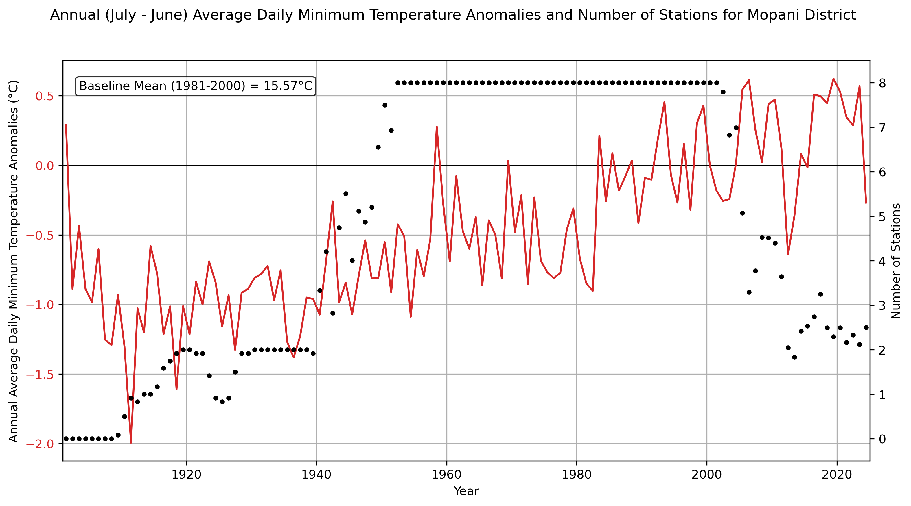
Daily Minimum Temperature (Tmin): The average is 15.6°C (Fig. 6). Similarly, there is variability and a suggested warming trend.
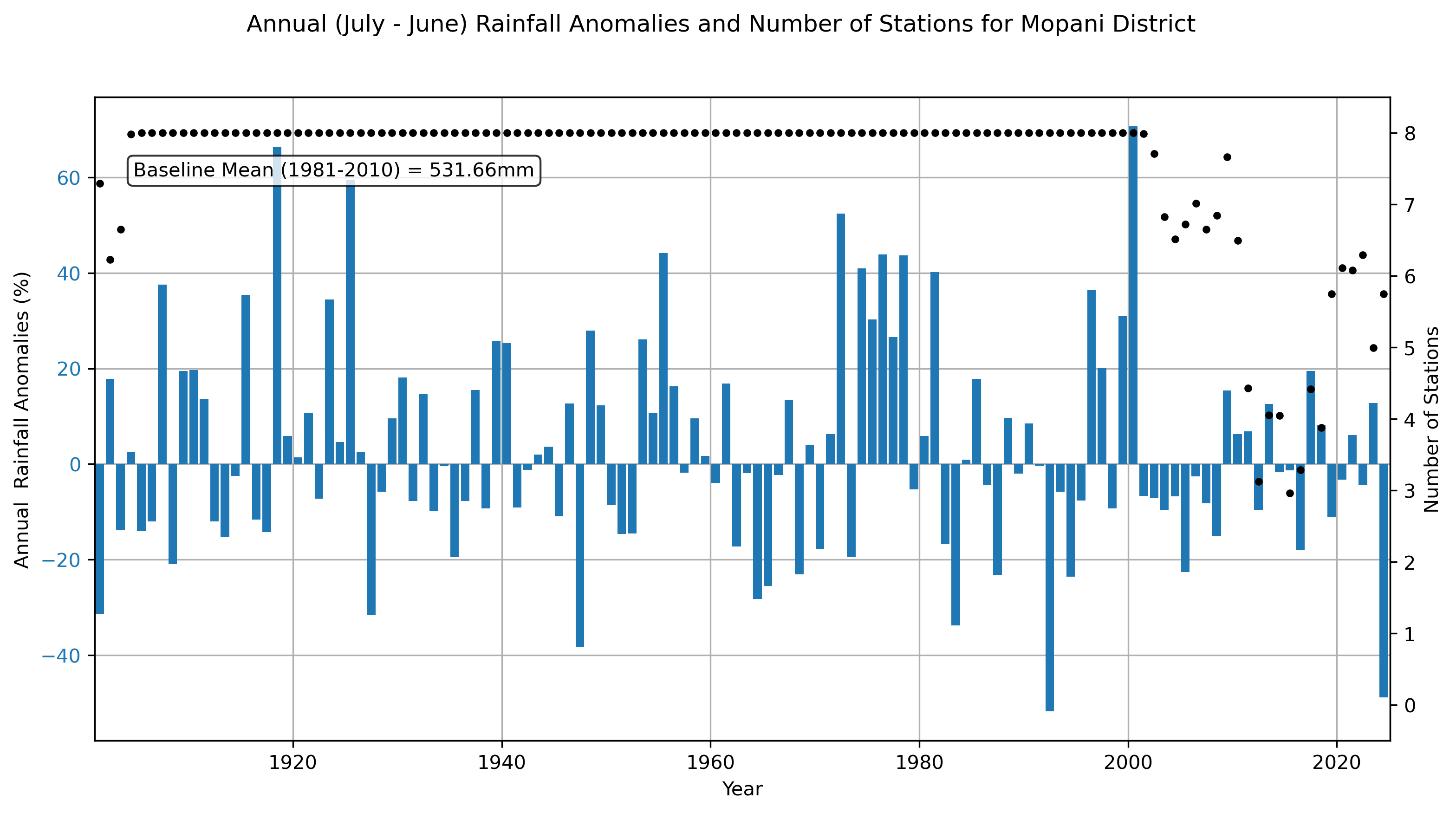
Annual Rainfall: The mean total rainfall is approximately 532 mm. The record shows strong interannual variability with multi-year wet or dry spells, but no clear long-term trend.
Note: South Africa historically maintained dense rainfall, and to a lesser extent temperature, station networks operated by the South African Weather Service, the Agricultural Research Council and other organisations. The data for these networks were combined and made freely available in 2000. This is the key reason for the high density of stations being utilized in the CRU dataset during the period 1904 - 2001 for rainfall and for 1951-2001 for the temperatures. The number of operational weather stations has decreased significantly during the last few decades and only a few of these stations make their data available to be used in datasets like CRU.
Advice to users
In this example, the user is advised not to use the temperature data for the period pre-1951 since very few station records are used to calculate the values. Also, there are no other sources of observed climate data against which to evaluate the skill of this dataset during this period. The data for most recent decades should be used with caution and the user is advised to evaluate the dataset against other available datasets.
The rainfall dataset may be used since the maximum number of stations are utilised for the majority of the period. Rainfall, and especially convective rainfall, is highly localized and episodic. Therefore the proximity of the stations to the target location is far more critical in comparison to temperature which is far more spatially and temporally consistent. CRU does not provide the exact location of the stations and therefore it is still advised to evaluate the dataset against other datasets, especially for the more recent decades.
Fig. 5: CRU TS annual (July - June) average daily maximum temperature anomalies and number of stations for the Mopani District (average gridcell values for domain lon 30 - 32, lat -24.5 - -23) for the period 1901-2023.
Fig. 6: CRU TS annual (July - June) average daily minimum temperature anomalies and number of stations for the Mopani District (average gridcell values for domain lon 30 - 32, lat -24.5 - -23) for the period 1901-2023.
Fig. 7: CRU TS annual (July - June) total rainfall anomalies (%) and number of stations for the Mopani District (average gridcell values for domain lon 30 - 32, lat -24.5 - -23) for the period 1901-2023.
The CRU TS mean annual total rainfall over this Mopani District is around 532 mm. It shows strong year to year variability, with some longer periods of above or below average rainfall. No clear trends in the rainfall are evident.
South Africa historically had an extensive rainfall station network and this is evidenced by the maximum number of stations being used to calculate this dataset for this region from 1904 - 2001. The decrease in station count post 2001 is due to both the reduction in active weather stations, but also in the number of stations that make their data available for use in datasets like CRU TS. The user is advised to evaluate the dataset against other datasets, especially for the more recent decades.
How can this data be used in disease modelling?
Malaria exhibits marked seasonality, characterised by cyclical increases in transmission intensity. Incidence tends to peak during the rainy season, which spans approximately from October to April across much of southern Africa. This seasonal amplification is largely driven by climatic conditions that enhance Anopheles vector survival, breeding site availability, and parasite development rates, collectively contributing to increased vector density and transmission potential.
Preparing the data
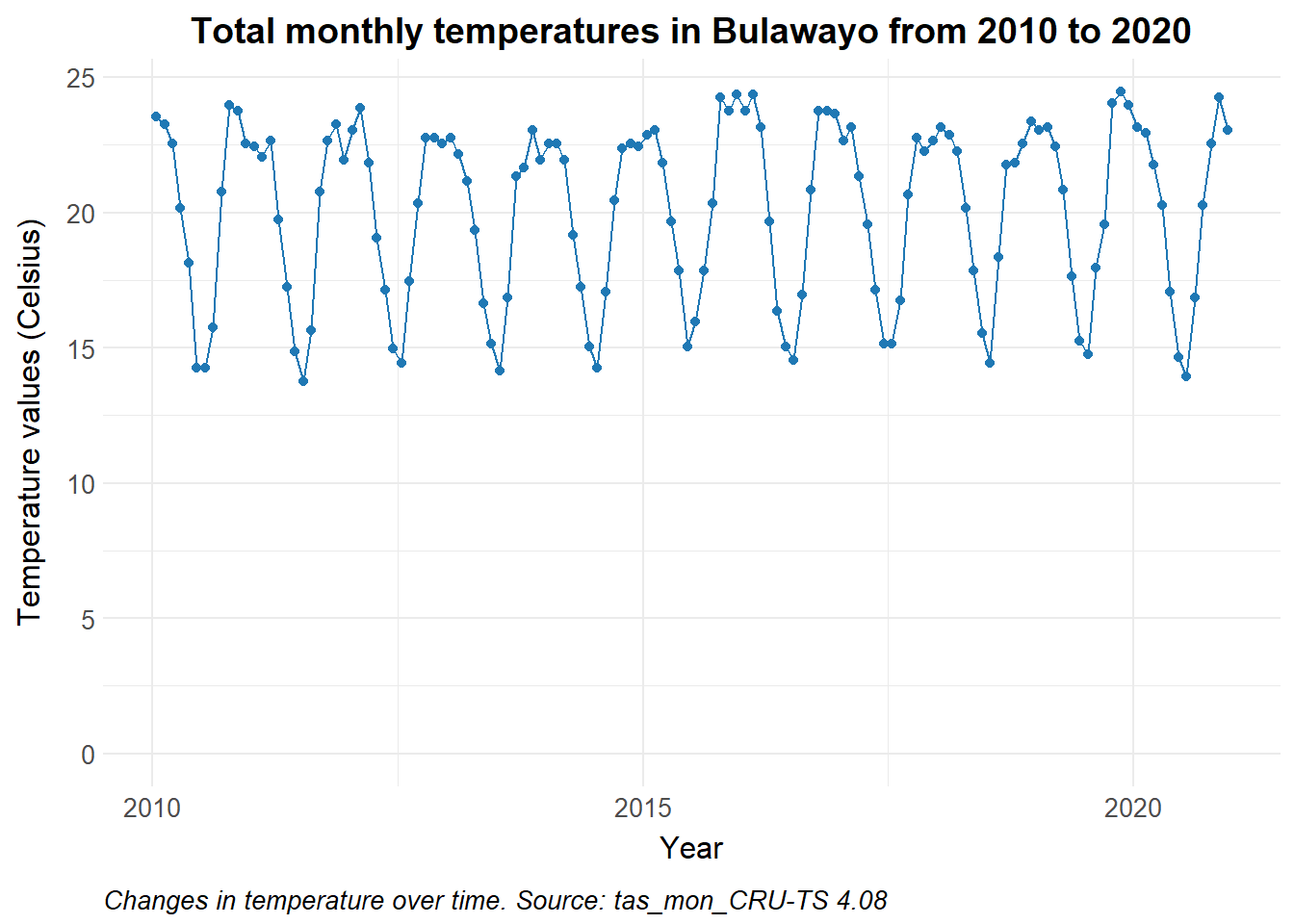
Using the CRU TS dataset, we obtain specific values for temperature over time, and model the historic impact of climatology on the vector population and subsequent incidence. We use mean air temperature as a proxy for surface temperatures.
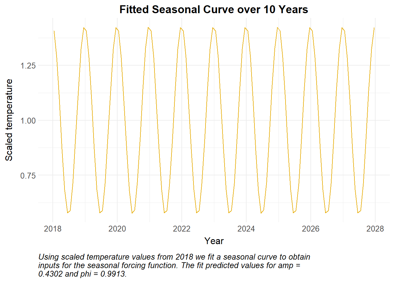
There are different approaches to include environmental conditions into an infectious disease model. In this example, we use the temperature data from Bulawayo to develop a seasonal forcing function that mimics the seasonal pattern of malaria transmission. We achieve this with the following cossine function, and fit it to the data to obtain the values of the amplitude of the peak and of (the phase angle that indicates timing of the peak): \[
1 + amp \times cos(2 \pi \times (\frac{time}{365} - \phi))
\]
You may need to adjust the function based on the transmission pattern in different contexts. Some countries may have more bimodal transmission (two peaks), a wide flat plateau, or many irregularly spaced peaks per year.
Show the code
# Load the data temperature_values <-read_csv("data/Fig5_tas_mon_CRU_TS-4.08_190101-202312_Bulawayo.csv") |>select(time, tas) |>mutate(tas = tas-273) |>#convert from Kelvin to Celsiusfilter(time >=ymd("2010-01-01") & time <=ymd("2020-12-31")) # start date of dataggplot() +geom_line(data = temperature_values, aes(x = time, y = tas), colour = theme_health_radar_colours[8]) +geom_point(data = temperature_values, aes(x = time, y = tas), colour = theme_health_radar_colours[8]) +theme_health_radar() +scale_colour_manual_health_radar() +labs(title ="Total monthly temperatures in Bulawayo from 2010 to 2020",x ="Year",y ="Temperature values (Celsius)",caption =str_wrap("Changes in temperature over time. Source: tas_mon_CRU-TS 4.08") ) +theme(legend.position ="none") +ylim(0, NA)
Show the code
# Convert one year of temperature data into seasonal forcing function by normalisation of valuestemperature_10yrs <-map_dfr(0:9, function(i) { temperature_values |>filter(time >=ymd("2018-01-01") & time <=ymd("2018-12-31")) |>arrange(time) |>mutate(scaled_rain = (tas -min(tas)) / (max(tas) -min(tas)),synthetic_time = time +years(i),year = i +1 )})# Fit cosine modelfit_data <- temperature_10yrs |>mutate(times =yday(synthetic_time), # add day-of-yeary = scaled_rain )fit <-nls( y ~1+ amp *cos(2* pi * (times /365- phi)), # seasonal forcing functiondata = fit_data,start =list(amp =0.5, phi =0.8) # choose starting values)#summary(fit) # look at values for amp and phi# Combine with initial datatemperature_10yrs <- temperature_10yrs |>mutate(times =yday(synthetic_time),predicted =predict(fit, newdata =data.frame(times =yday(synthetic_time))) # predict from fit )temperature_10yrs |>ggplot() +geom_line(aes(x = synthetic_time, y = predicted), colour = theme_health_radar_colours[6], show.legend = F) +labs(title ="Fitted Seasonal Curve over 10 Years",x ="Year", y ="Scaled temperature",caption =str_wrap("Using scaled temperature values from 2018 we fit a seasonal curve to obtain inputs for the seasonal forcing function. The fit predicted values for amp = 0.4302 and phi = 0.9913.") ) +theme_health_radar()
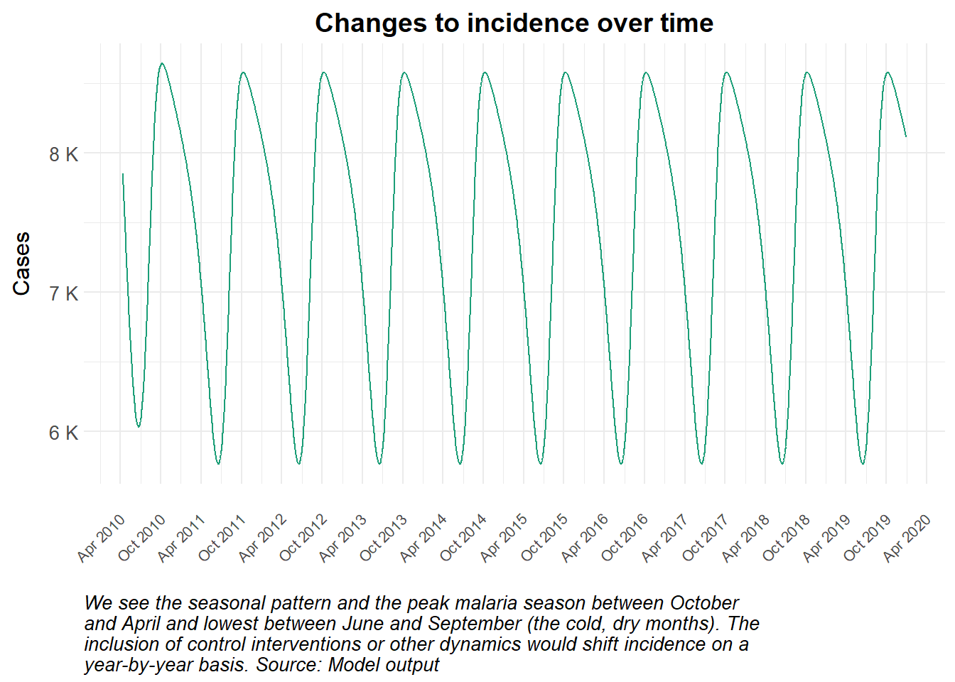
We incorporate this into the model to see the seasonal pattern in incidence.
Show the code
# Time points for the simulationY =10# Years of simulationtimes <-seq(0, 365*Y, by =1)# SEACR-SEI modelseacr <-function(times, start, parameters) { with(as.list(c(start, parameters)), { P = S + E + A + C + R + G M = Sm + Em + Im m = M / P# Seasonality seas =1+amp*cos(2*pi*(times/365- phi))# Force of infection Infectious = C + zeta_a*A #infectious reservoir lambda.v <- seas*a*M/P*b*Im/M lambda.h <- seas*a*c*Infectious/P# Differential equations/rate of change dSm = mu_m*M - lambda.h*Sm - mu_m*Sm dEm = lambda.h*Sm - (gamma_m + mu_m)*Em dIm = gamma_m*Em - mu_m*Im dS = mu_h*P - lambda.v*S + rho*R - mu_h*S dE = lambda.v*S - (gamma_h + mu_h)*E dA = pa*gamma_h*E + pa*gamma_h*G - (delta + mu_h)*A dC = (1-pa)*gamma_h*E + (1-pa)*gamma_h*G - (r + mu_h)*C dR = delta*A + r*C - (lambda.v + rho + mu_h)*R dG = lambda.v*R - (gamma_h + mu_h)*G dCInc = lambda.v*(S+R)# Outputlist(c(dSm, dEm, dIm, dS, dE, dA, dC, dR, dG, dCInc)) })}# Initial values for compartments(approximations for Bulawayo, Zimbabwe)initial_state <-c(Sm =1000000, # susceptible mosquitoesEm =100000, # exposed and infected mosquitoesIm =200000, # infectious mosquitoesS =350000, # susceptible humansE =35000, # exposed and infected humansA =130000, # asymptomatic and infectious humansC =65000, # clinical and symptomatic humansR =100000, # recovered and semi-immune humansG =10000, # secondary-exposed and infected humansCInc =0# cumulative incidence)# Country-specific parameters should be obtained from literature review and expert knowledgeparameters <-c(a =0.45, # human biting rateb =0.5, # probability of transmission from mosquito to humanc =0.6, # probability of transmission from human to mosquitor =1/21, # rate of loss of infectiousness after treatmentrho =1/160, # rate of loss of immunity after recoverydelta =1/150, # natural recovery ratezeta_a =0.4, # relative infectiousness of of asymptomatic infectionspa =0.4, # probability of asymptomatic infectionmu_m =1/10, # birth and death rate of mosquitoesmu_h =1/(62*365), # birth and death rate of humansgamma_m =1/10, # extrinsic incubation rate of parasite in mosquitoesgamma_h =1/10, # extrinsic incubation rate of parasite in humansamp =0.4302, # amplitude of seasonalityphi =0.9913# phase angle, start of season )# Run the modelout <-ode(y = initial_state, times = times, func = seacr, parms = parameters)# Post-processing model output into a dataframedf <-as_tibble(as.data.frame(out)) |>mutate(P = S + E + A + C + R + G,M = Sm + Em + Im,Inc =c(0, diff(CInc))) |>pivot_longer(cols =-time, names_to ="variable", values_to ="value") |>mutate(date =ymd("2010-01-01") + time)df |>filter(variable =="Inc", time >100) |>ggplot() +geom_line(aes(x = date, y = value, colour = variable), show.legend = F) +theme_health_radar() +theme(axis.text.x =element_text(angle =45, hjust =1, size =8)) +scale_colour_manual_health_radar() +scale_y_continuous(labels = scales::label_number(suffix =" K", scale =1e-3)) +scale_x_date(date_labels ="%b %Y",date_breaks ="6 months") +labs(title ="Changes to incidence over time", x =" ",y ="Cases",colour ="Population",caption =str_wrap("We see the seasonal pattern and the peak malaria season between October and April and lowest between June and September (the cold, dry months). The inclusion of control interventions or other dynamics would shift incidence on a year-by-year basis. Source: Model output") )
Policy implications
Incorporating time-varying transmission into the model reflects the real-world seasonality of malaria. This can be used to plan the timing of interventions, aligning delivery to the peak of the season across different geographical regions. These differences in risk (across geographic regions and seasons) are also important insights for resource allocation and health systems planning, ensuring consistent access to care and other control measures.
This model uses a seasonal forcing function as opposed to explicit climatic data, and as such the model does not capture details such as extreme weather events, such as 2017’s Cyclone Dineo (which may have contributed to increases in malaria cases across southern Africa) or other long-term periodic climatic phenomena such as the El Niño-Southern Oscillation (ENSO) cycle. We show the explicit use of temperature and rainfall using ERA5 data here.
In climate science, the skill of a dataset refers to its accuracy, resolution, bias, uncertainty, and predictive power in representing real-world climate conditions. A high-skill dataset closely matches observations, has minimal bias, and reliably supports climate modelling and decision-making↩︎