The DHS (Demographic and Health Surveys) Program provides data on population, health, and nutrition through more than 400 surveys in over 90 countries. Data covers the following areas; Population and Demographics, Fertility and Family Planning, Maternal and Child Health, Nutrition, HIV/AIDS and Other Infections, Malaria, & Gender and Domestic Violence.
The DHS data are widely used by governments, NGOs, researchers, and policymakers to design and monitor health programs and policies. The surveys are conducted through face-to-face interviews with representative samples of households, and they use standardized questionnaires to ensure comparability across countries and over time.
Demographic health surveys are also unique for modelling as you can correlate across various datasets variables for example linking Malaria data on prevention and treatment to other factors in the population and demographics data to other health system indicators
Accessing the data
There are several options for accessing the data, each thoroughly explained in other resources.
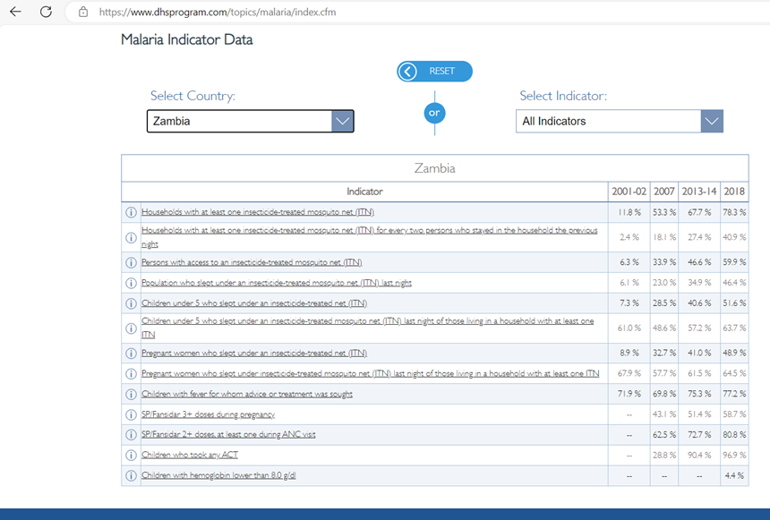
STATcompiler, a graphical user interface tool for accessing and downloading the data in CSV format.
Accessing the data using STATcompiler
Prevalence and Treatment: Users can access data on malaria prevalence and treatment practices directly from the STATcompiler. It allows for the creation of tables, charts, and maps that display malaria prevalence rates, treatment practices, and trends over time.
Preventive Measures: STATcompiler provides data on the ownership and use of ITNs, IRS coverage, and IPTp usage. Users can visualize how these preventive measures vary across different regions and demographic groups.
Country and Regional Comparisons: STATcompiler enables users to compare malaria data across different countries and regions. This comparative analysis helps in identifying best practices and areas that require more attention.
Temporal Trends: Users can analyze trends over time to see how malaria prevention and treatment efforts have evolved and their impact on malaria prevalence and morbidity
Tailored Data Retrieval: STATcompiler allows users to create custom tables based on specific indicators related to malaria. Users can filter data by variables such as age, sex, urban/rural residence, and wealth quintile.
Indicator Selection: Users can select specific indicators related to malaria, such as ITN usage, malaria prevalence among children under five, and access to malaria treatment. This customization helps in focusing on particular aspects of malaria control and prevention.
Holistic Health Analysis: STATcompiler can integrate malaria data with other health indicators, such as child mortality rates, nutrition status, and maternal health. This integration provides a comprehensive view of health challenges and the interconnections between different health issues.
Multi-Indicator Analysis: Users can analyse how malaria prevention and treatment efforts correlate with other health outcomes, facilitating a broader understanding of health dynamics.
Interactive Tools: STATcompiler offers an interactive and user-friendly interface, making it easy for users to navigate and extract relevant malaria data.
Data Export: Users can export data in various formats (e.g., Excel, CSV) for further analysis or reporting purposes.
Practical Applications using STATcompiler to access DHS program data
Policy Making and Program Design: Policymakers and program designers can access up-to-date malaria data, helping them create evidence-based strategies and allocate resources effectively.
Research and Academic Studies: Researchers can utilize STATcompiler to obtain detailed malaria data for their studies, facilitating in-depth analysis and publication of findings.
Monitoring and Evaluation: Health organizations can monitor the progress of malaria interventions by analysing trends and identifying gaps in coverage .
By leveraging the capabilities of STATcompiler, users can efficiently analyse and visualise malaria data collected by the DHS Program, leading to more informed decisions and effective interventions in malaria control and prevention.
The Demographic and Health Surveys (DHS) Program has developed an open-source R package rdhs for management and analysis of Demographic and Health Survey data. This includes functionality to:
indicators <-dhs_indicators()# Find all indicators starting with MLall_malaria_indicators = indicators[grepl("^ML", indicators$IndicatorId), c("IndicatorId", "Definition")]knitr::kable(head(all_malaria_indicators))
IndicatorId
Definition
2269
ML_NETP_H_MOS
Percentage of households with at least one mosquito net (treated or untreated)
2270
ML_NETP_H_ITN
Percentage of households with at least one insecticide treated mosquito net (ITN)
2271
ML_NETP_H_LLN
Percentage of households with at least one long-lasting insecticide treated mosquito net (LLIN)
2272
ML_NETP_H_MNM
Mean number of mosquito nets per household
2273
ML_NETP_H_MNI
Mean number of insecticide tested mosquito nets (ITNs) per household
2274
ML_NETP_H_MNL
Mean number of long-lasting insecticide tested mosquito nets (LLINs) per household
Show the code
tags <-dhs_tags()# Get the tags related to malariaknitr::kable(tags[grepl("Malaria", tags$TagName), ])
TagType
TagName
TagID
TagOrder
33
0
Malaria Parasitemia
36
540
45
2
Select Malaria Indicators
79
1000
Show the code
# Get the country codes of the frontline 4 of the elimination 8 countriesall_countries =dhs_countries(returnFields=c("CountryName","DHS_CountryCode"))# Get the country codes of the frontline 4 of the elimination 8 countriesfrontline4 =c("Botswana", "Namibia", "South Africa", "Eswatini")elim8 =c("Botswana", "Namibia", "South Africa", "Eswatini", "Zambia", "Zimbabwe", "Mozambique", "Malawi")# Get the country codes of the frontline 4 of the elimination 8 countriesf4_codes = all_countries[all_countries$CountryName %in% frontline4, "DHS_CountryCode"]e8_codes = all_countries[all_countries$CountryName %in% elim8, "DHS_CountryCode"]# Retrieve DHS data for the specified indicator, countries, and survey yearsdata1 <-dhs_data(indicatorIds ="ML_NETP_H_MOS",countryIds = f4_codes,surveyYearStart =2000,breakdown ="subnational")# Remove rows with CharacteristicLabel starting with ".." to avoid double counting regionsfilt_data = data1[!grepl("^\\..*", data1$CharacteristicLabel),]# Filter the data for Namibia onlyfilt_data = filt_data[filt_data$CountryName =="Namibia",]
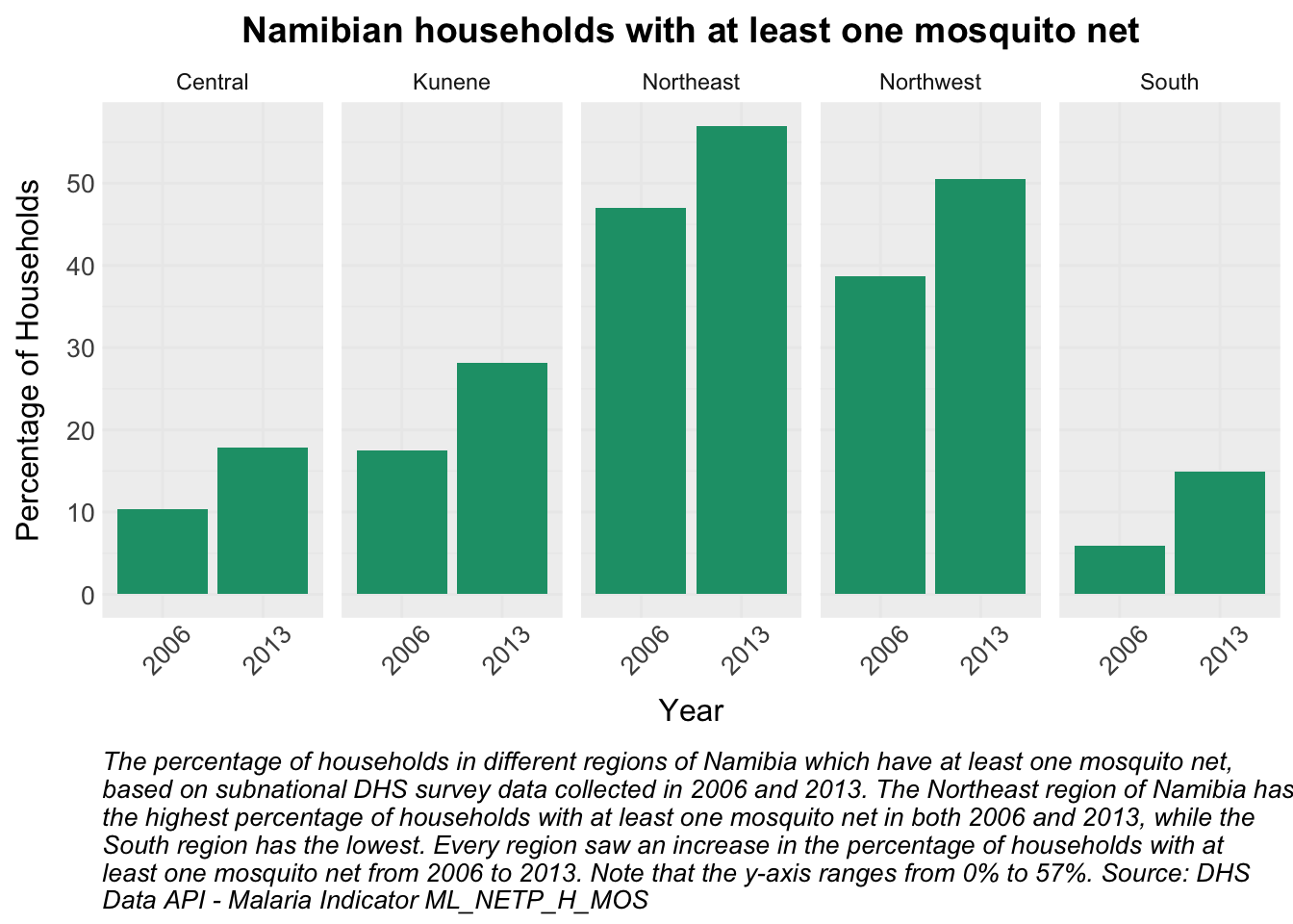
A faceted bar plot can be used to visualise the percentage of households with at least one insecticide-treated net (ITN) in each Namibian province at a small number of time points.
Show the code
# Define a single color for the barssingle_color <-"#1b9e77"# Plot the data as a bar plotggplot(filt_data, aes(x =as.factor(SurveyYear), y = Value, fill = single_color)) +# Create bar plot with identity statistic and no legendgeom_bar(stat ="identity", position ="dodge", show.legend =FALSE) +# Use the health radar color schemescale_fill_manual_health_radar() +# Set y-axis ticks increment to 10scale_y_continuous(breaks =seq(0, max(filt_data$Value, na.rm =TRUE), by =10)) +# Facet the plot by CharacteristicLabel, with 6 columnsfacet_wrap(~ CharacteristicLabel, ncol =6) +# Apply the health radar themetheme_health_radar() +# Additional theme customizations specific to this plottheme(axis.text.x =element_text(angle =45, hjust =0.4),legend.position ="none",panel.background =element_rect(fill ="#F0F0F0", color =NA),panel.spacing =unit(0.5, "lines")) +# Add titles and labelslabs(title ="Namibian households with at least one mosquito net",x ="Year",y ="Percentage of Households",caption =str_wrap("The percentage of households in different regions of Namibia which have at least one mosquito net, based on subnational DHS survey data collected in 2006 and 2013. The Northeast region of Namibia has the highest percentage of households with at least one mosquito net in both 2006 and 2013, while the South region has the lowest. Every region saw an increase in the percentage of households with at least one mosquito net from 2006 to 2013. Note that the y-axis ranges from 0% to 57%. Source: DHS Data API - Malaria Indicator ML_NETP_H_MOS", width =100))
Show the code
# Retrieve DHS data for the specified indicator, countries, and survey yearsdata2 <-dhs_data(indicatorIds ="ML_NETP_H_MNM",countryIds = e8_codes,surveyYearStart =2000,breakdown ="subnational")# Keep only the rows where the level rank is 1 (national level data)filt_data = data2[data2$LevelRank ==1,]# Remove rows with CharacteristicLabel starting with ".." to avoid double counting regionsfilt_data = filt_data[!grepl("^\\..*", filt_data$CharacteristicLabel),]
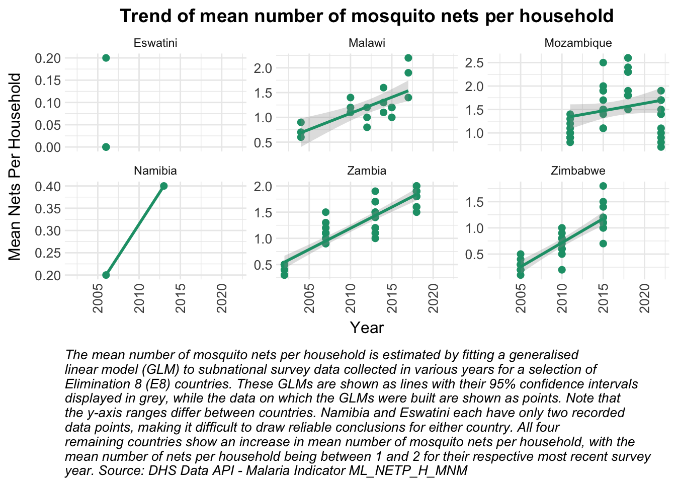
Generalised linear models can be used to fit an estimated mean value for the number of mosquito nets per household in various African countries. Rather than including all of these countries on one plot, the visualisation can be faceted to show multiple smaller plots - one for each country.
Show the code
# Plot the data using ggplot2ggplot(filt_data, aes(x = SurveyYear, y = Value), colour = single_color) +# Add points to the plotgeom_point(size =2, colour = single_color) +# Add a smooth line using a generalised linear model, with confidence interval shadinggeom_smooth(method ="glm", se =TRUE, alpha =0.3, colour = single_color) +# Facet the plot by CountryName, with 3 columns and free y-axis scalesfacet_wrap(~ CountryName, ncol =3, scales ="free_y") +# Apply the health radar theme and colorstheme_health_radar() +scale_colour_manual_health_radar() +# Additional theme customizations specific to this plottheme(axis.text.x =element_text(angle =90, vjust =0.5) ) +# Center the legend titleguides(colour =guide_legend(title.position ="top", title.hjust =0.5)) +# Add titles and labelslabs(title ="Trend of mean number of mosquito nets per household",x ="Year",y ="Mean Nets Per Household",caption =str_wrap("The mean number of mosquito nets per household is estimated by fitting a generalised linear model (GLM) to subnational survey data collected in various years for a selection of Elimination 8 (E8) countries. These GLMs are shown as lines with their 95% confidence intervals displayed in grey, while the data on which the GLMs were built are shown as points. Note that the y-axis ranges differ between countries. Namibia and Eswatini each have only two recorded data points, making it difficult to draw reliable conclusions for either country. All four remaining countries show an increase in mean number of mosquito nets per household, with the mean number of nets per household being between 1 and 2 for their respective most recent survey year. Source: DHS Data API - Malaria Indicator ML_NETP_H_MNM", width =95) )
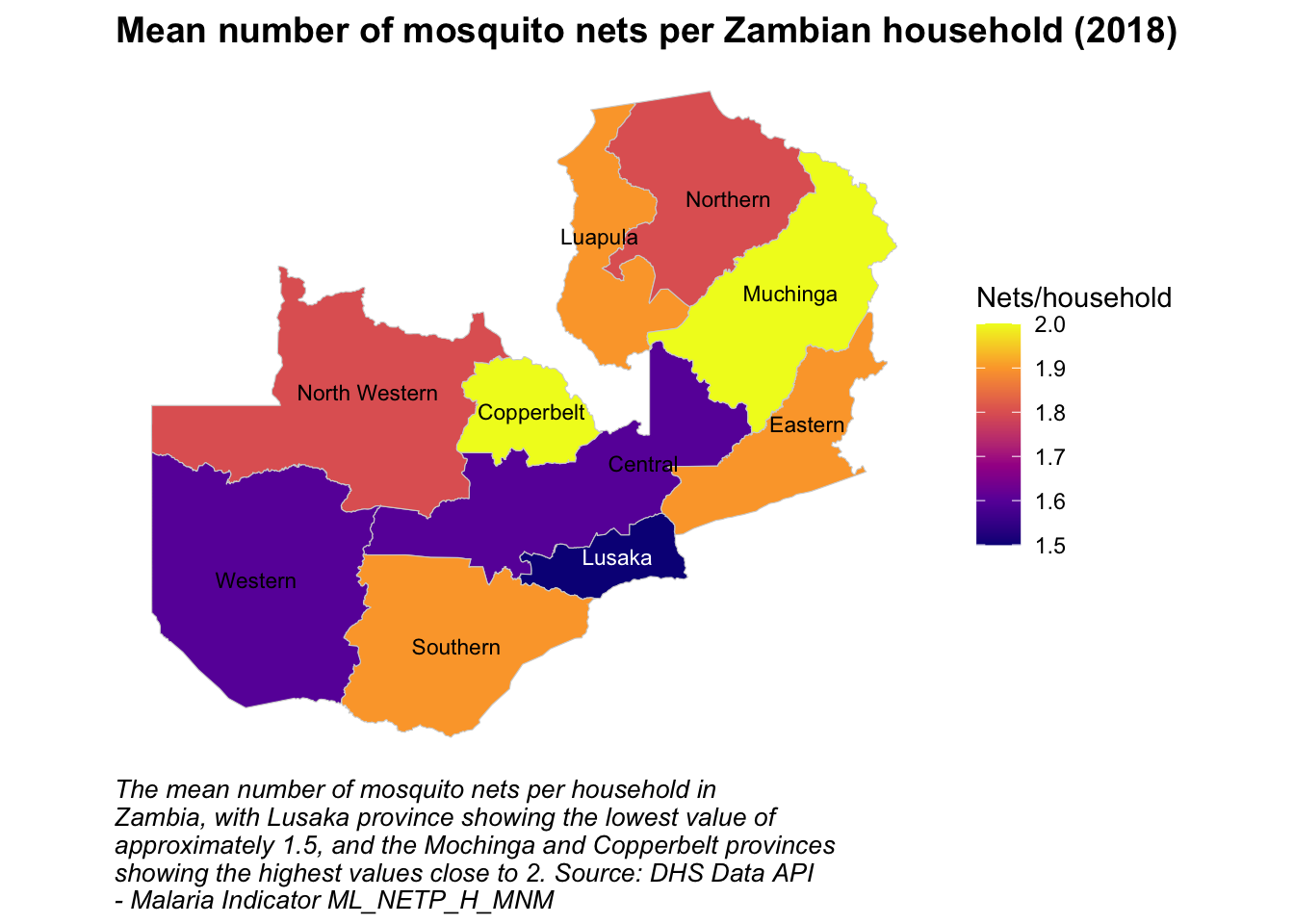
A map is an effective method of visualising the mean number of mosquito nets per Zambian province.
Show the code
# Filter the data for Zambia for the year 2018d = data2[(data2$CountryName =="Zambia"& data2$SurveyYear ==2018),]# Download the related spatial data frame object for Zambiasp <-download_boundaries(surveyId = d$SurveyId[1], method ="sf")# Match our values to the regions in the spatial datam <- d$Value[match(sp$sdr_subnational_boundaries$REG_ID, d$RegionId)]sp$sdr_subnational_boundaries$Value <- m# Plot the spatial data using ggplot2ggplot(sp$sdr_subnational_boundaries) +# Add a filled polygon layer for each regiongeom_sf(aes(fill = Value), color ="lightgrey", size =0.3) +# Use the health radar continuous color scale for the fillscale_fill_continuous_health_radar(option ="plasma", na.value ="grey50", name ="Nets/household") +# Add titles and labelslabs(title ="Mean number of mosquito nets per Zambian household (2018)",caption =str_wrap("The mean number of mosquito nets per household in Zambia, with Lusaka province showing the lowest value of approximately 1.5, and the Mochinga and Copperbelt provinces showing the highest values close to 2. Source: DHS Data API - Malaria Indicator ML_NETP_H_MNM", width =60)) +# Conditional text colorgeom_sf_text(aes(label = DHSREGEN, color =ifelse(Value >quantile(Value, 0.1), "black", "white")), size =3) +scale_color_identity() +# Apply the health radar themetheme_health_radar() +# Remove x- and y-axes and grid linestheme(plot.title.position ="plot",axis.title.x=element_blank(),axis.text.x=element_blank(),axis.ticks.x=element_blank(),axis.title.y=element_blank(),axis.text.y=element_blank(),axis.ticks.y=element_blank(),panel.grid.major =element_blank(), panel.grid.minor =element_blank())
An example of a more interactive mapped visualisation, this time of Malawi rather than Zambia, is shown below.
Show the code
library(leaflet)# Make a request to DHS data API for Malawi, for the specified indicator, and survey yearsd2 <-dhs_data(countryIds ="MW",indicatorIds ="ML_FEVT_C_AML",breakdown ="subnational",surveyYearStart =2016,returnGeometry =TRUE,f ="geojson")# Convert the retrieved data to JSON formatm <- geojsonio::as.json(d2)# Convert the JSON data to a spatial objectnc2 <- geojsonio::geojson_sp(m) # Create a color palette using the health radar colors for continuous data# Using the first few colors from theme_health_radar_colours for the gradientpal <- leaflet::colorNumeric(palette =colorRampPalette(theme_health_radar_colours[1:3])(100),domain = nc2$Value,na.color ="grey50")# Plot the data using leafletleaflet(nc2[nc2$IndicatorId =="ML_FEVT_C_AML", ]) %>%# Add base map tilesaddTiles() %>%# Add polygons to represent the regionsaddPolygons(stroke =TRUE,color = theme_health_radar_colours[7], # Using the grey from our themeweight =0.5,smoothFactor =0.3,fillOpacity =0.8,fillColor =~pal(Value),# Add labels to the polygons with characteristic label and valuelabel =~paste0(CharacteristicLabel, ": ", formatC(Value, big.mark =",")),labelOptions = leaflet::labelOptions(style =list("font-weight"="bold","color"= theme_health_radar_colours[7] # Using theme color for labels ),textsize ="13px",direction ="auto" ) ) %>%# Add a legend to the mapaddLegend(pal = pal,values =~Value,opacity =1.0,title ="Malawi: children with fever who took antimalarial drugs (%)",position ="bottomright",labFormat =labelFormat() ) %>%# Set the initial view of the map to focus on MalawisetView(lng =37, lat =-13, zoom =5.5)
How can this data be used in disease modelling?
The DHS dataset has various components that can be incorporated into malaria modelling, particularly with respect to health systems and interventions. Upon exploring the data, many indicators from the DHS surveys may be associated with the system dynamics of malaria. We include a few examples below:
Number of children age 6-59 months tested for malaria using microscopy
Percentage of pregnant women who slept under a long-lasting insecticide treated net (LLIN) the night before the survey
Among children with fever in the two weeks preceding the survey for whom advice or treatment was sought, the percentage for whom the source was a government health center, traditional practitioner, shop or private doctor
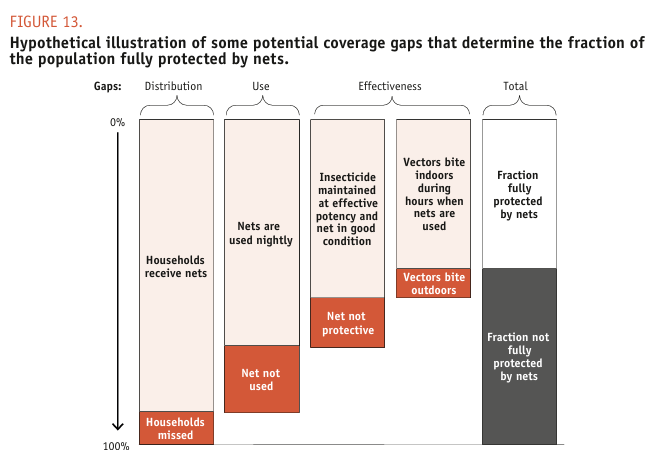
In modelling LLIN effective coverage, we account for the number of households that actually receive nets, appropriate usage, insecticide efficacy and the physical integrity of the net. Human and vector behavioural characteristics pertaining to where people spending their evenings (during peak biting times), or the likelihood of indoor vector biting are captured as operational effectiveness\(opp_{eff}\). Another illustration of this is depicted below:
Source: WHO (2014). From malaria control to malaria elimination: a manual for elimination scenario planning.
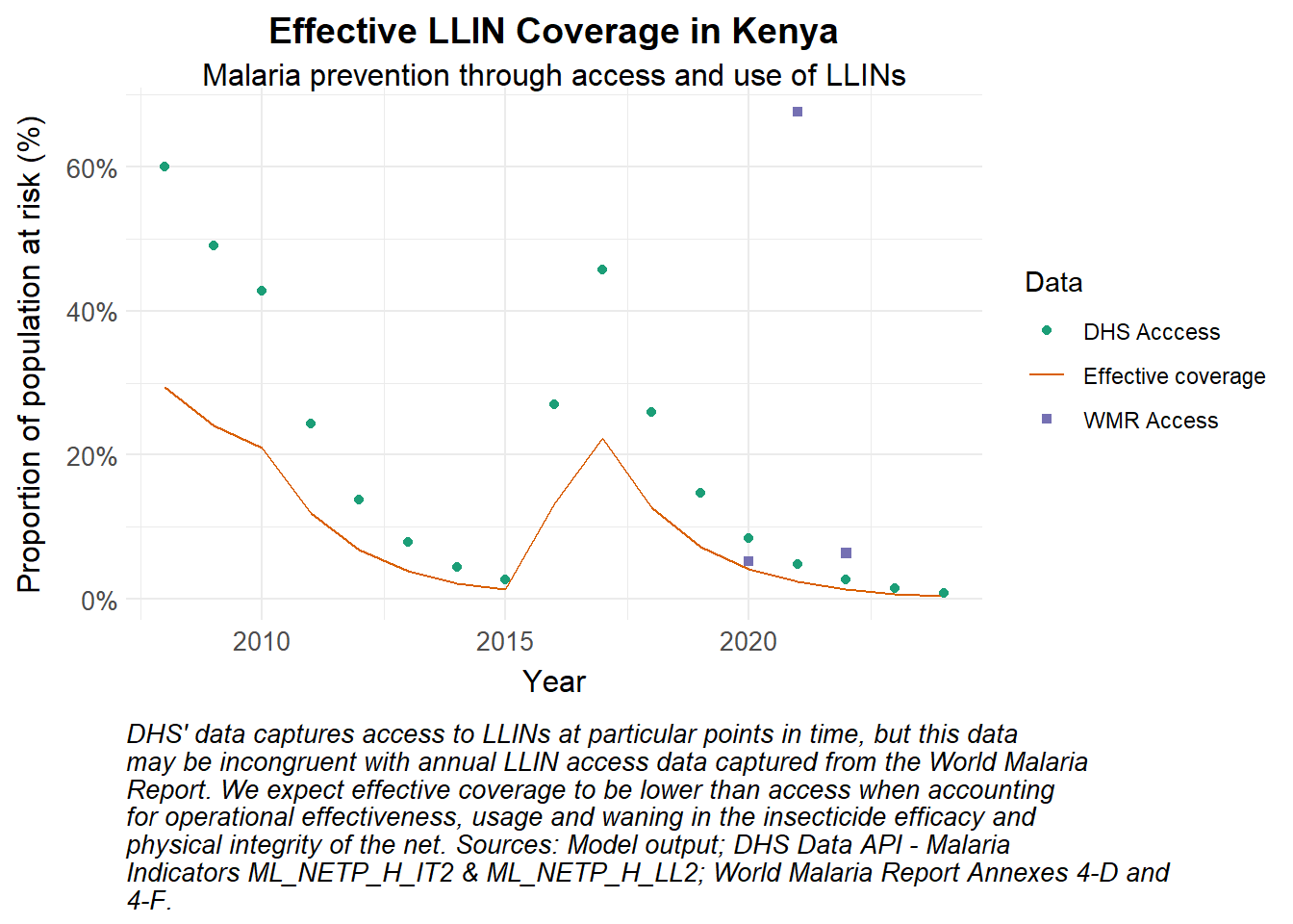
In the simple example below, we obtain data on LLIN access and usage rates in Kenya from the DHS, and compare this to data on ITN distribution from the World Malaria Report. Finally, we model the effective coverage of LLINs. This represents the proportion of the population actually protected from malaria transmission by LLINs in a particular country.
Preparing the data
The relevant indicators are sourced from the DHS datasets.
Show the code
## Source LLIN coverage and usage data from DHSindicators <-dhs_indicators()all_malaria_indicators <- indicators |>filter(Level1 =="Malaria") |>select(c("IndicatorId", "Definition"))# Select DHS indicators# ML_NETP_H_LL2: Percentage of households with at least one long-lasting insecticidal net (LLIN) for every two persons who stayed in the household the previous night# ML_ITNU_N_ITN: Percentage of existing insecticide treated nets used the night before the surveyaccess_data <-dhs_data(indicatorIds ="ML_NETP_H_LL2",countryIds ="KE")usage_data <-dhs_data(indicatorIds ="ML_ITNU_N_ITN",countryIds ="KE")# Obtain LLIN access and usage dataLLIN_access <- access_data |>arrange(SurveyYear) |>select(SurveyYear, Value) |>complete(SurveyYear =full_seq(c(SurveyYear, 2024), 1), fill =list(Value =0)) |>mutate(time =seq(365, 365*17, by =365)) |># 17 years of simulationmutate(access = Value/100)LLIN_data <- usage_data |>arrange(SurveyYear) |>select(SurveyYear, Value) |>complete(SurveyYear =full_seq(c(SurveyYear, 2024), 1)) |>fill(Value, .direction ="down") |>mutate(usage = Value/100)# Merge the two datasetsLLIN_data <-full_join(LLIN_data, LLIN_access, by ="SurveyYear") |>filter(SurveyYear >2007)
Model assumptions
We make a few assumptions about LLINs in the model, explicitly stated here. We assume:
Net usage remains consistent until a new survey is conducted.
Net functionality and effectiveness declines at a rate of approximately 25% per year, with LLINs considered ‘expired’ or no longer effective after three years of use.”
Would you like to expand this into a p
Operational effectiveness (\(opp_{eff}\)): 65% of actual bites from an indoor-biting infectious mosquito are assumed to be prevented by LLINs used correctly during peak biting times.
Coverage
Coverage is dependent on access to LLINs at the distribution rate of two persons per net. The reported number of ITNs distributed in a given year in each country can be obtained from the World Malaria Report Annex 4-D.
\[
\textrm {Access} = \frac {\textrm{Nets distributed} \times 2}{\textrm {Population at risk}} - \textrm {losses due to insecticide decay and physical wear and tear}
\tag{1}\]
Subsequently, effective coverage can be quite low due to imperfect usage and operational effectiveness.
The timelines of the datasets do not align: DHS survey data on LLIN access are available for the years 2008, 2014, and 2015, while net usage data are available for 2008, 2014, 2015, 2020, and 2022. The World Malaria Report provides LLIN access values only for the three years preceding the 2023 report. Nonetheless, we present both LLIN access values and the calculated effective coverage in the same figure below for illustrative purposes.
Show the code
library(deSolve)# Time points for the simulationY =17# Years of simulationtimes <-seq(0, 365*Y, 1) # time in days# Define LLIN model ####itnmod <-function(times, start, parameters) {with(as.list(c(parameters, start)), { llin_time <- LLIN_data$time llin_access <-approx(llin_time, LLIN_data$access, times, method ="constant", rule =2)$y usage <-approx(llin_time, LLIN_data$usage, times, method ="constant", rule =2)$y eta <--log(1-(att1-att3))/(3*365) # rate of loss due to attrition rate over three year period llin_eff_cov =min(LLIN,1)*usage*opp_eff dLLIN = llin_access/365- (eta + phi)*LLINlist(dLLIN, llin_eff_cov) })}# Input definitions ##### Initial valuesstart <-c(LLIN =0.6) # proportion of the population currently protected by LLINs in circulation# Parametersparameters <-c(opp_eff =0.65, # Operational effectiveness of LLIN at preventing transmissionatt1 =1, # proportion of nets distributed in year X circulating in year Xatt2 =0.75, # proportion of nets distributed in year X circulating in year X+1att3 =0.5, # proportion of nets distributed in year X circulating in year X+2phi =1/(3*365) # death rate of LLINS)# Run the modelout <-ode(y = start, times = times, func = itnmod, parms = parameters)model_output_df <-as_tibble(as.data.frame(out)) |>rename(llin_eff_cov =`2`) |>mutate(year =as.numeric(format(as.Date("2008-01-01") + time, "%Y"))) |>mutate(Data ="Effective coverage") |>group_by(year) |>slice_head(n =1) |># summarise by yearungroup()# Source access data from World Malaria Report## LLINs distributed annuallydist_data <- whowmr::wmr2023$wmr2023d |>filter(`Country/area`=="Kenya") |>select(Year, `No. of LLINs delivered`)## Population at riskWHO_data <- whowmr::wmr2023$wmr2023f |>filter(`Country/area`=="Kenya", Year >2007) |>select(Year, `Population denominator for incidence and mortality rate`)# Merge the two datasets and calculate access to LLINs in the population at riskWHO_data <-full_join(WHO_data, dist_data, by ="Year") |># add distribution data to same dataframemutate(Proportion_population =`No. of LLINs delivered`*2/`Population denominator for incidence and mortality rate`) |># one net per 2 persons at riskmutate(Data ="WMR Access")ggplot() +geom_line(data = model_output_df, aes(x = year, y = llin_eff_cov, colour = Data)) +geom_point(data = model_output_df |>mutate(Data ="DHS Acccess"), aes(x = year, y = LLIN, colour = Data)) +geom_point(data = WHO_data, aes(x = Year, y = Proportion_population, colour = Data), shape =15) +scale_y_continuous(labels = scales::percent) +theme_health_radar() +scale_colour_manual_health_radar() +labs(title ="Effective LLIN Coverage in Kenya" ,subtitle ="Malaria prevention through access and use of LLINs",x ="Year",y ="Proportion of population at risk (%)",caption =str_wrap("DHS' data captures access to LLINs at particular points in time, but this data may be incongruent with annual LLIN access data captured from the World Malaria Report. We expect effective coverage to be lower than access when accounting for operational effectiveness, usage and waning in the insecticide efficacy and physical integrity of the net. Sources: Model output; DHS Data API - Malaria Indicators ML_NETP_H_IT2 & ML_NETP_H_LL2; World Malaria Report Annexes 4-D and 4-F."))
Policy implications
Gaps between access to LLINs and actual effective coverage can justify increasing the frequency of mass distribution campaigns or implementing continuous distribution channels through schools and health clinics. Where these gaps stem from low usage rates, targeted social and behavioural change campaigns may be necessary to improve net use. Alternatively, if low effective coverage is due to vector insecticide resistance, switching to nets with different or enhanced active ingredients may prove to be a better strategy. In settings where human behaviour (spending evenings outdoors in fields, at taverns, or fishing) limits the operational effectiveness of LLINs, complementary strategies to address outdoor biting could be considered.