# Time points for the simulation
Y = 14 # Years of simulation
times <- seq(0, 365*Y, by = 1)
# Estimates of resistance levels over time
resdata <- insecticide_data_summ |>
filter(RESISTANCE_STATUS == "Confirmed resistance") |>
mutate(mean_mortality = mean_mortality/100) # convert into decimal
# Make a time dependent variable of resistance levels
effr_level <- approxfun(resdata$time, resdata$mean_mortality, n = 365*Y, ties = "ordered", method = "constant", rule = 2)
# SEACR-SEI model
seacr <- function(times, start, parameters, effr_level) {
with(as.list(c(start, parameters)), {
P = S + E + A + C + R + G
M_s = Sm_s + Em_s + Im_s
M_r = Sm_r + Em_r + Im_r
M = M_s + M_r
m = M / P
# Seasonality
seas.t <- amp*(1+cos(2*pi*(times/365-phi)))
# Nets
itn <- itn_cov*itn_use
itn_r <- itn*(effr_level(times)) # Adjust effective coverage of ITNs based on resistance level
# Force of infection
Infectious = C + zeta_a*A # infectious reservoir
lambda.v <- seas.t*a*M/P*b*(Im_r*(1-itn_r) + Im_s*(1-itn))/M
lambda.h <- seas.t*a*c*Infectious/P*(1-itn)
# Differential equations/rate of change
# Insecticide-sensitive mosquito compartments
dSm_s = (1-res)*mu_m*M - (lambda.h)*Sm_s - mu_m*Sm_s
dEm_s = (lambda.h)*Sm_s - (gamma_m + mu_m)*Em_s
dIm_s = gamma_m*Em_s - mu_m*Im_s
# Insecticide-resistant mosquito compartments
dSm_r = res*mu_m*M - (lambda.h)*Sm_r - mu_m*Sm_r
dEm_r = (lambda.h)*Sm_r - (gamma_m + mu_m)*Em_r
dIm_r = gamma_m*Em_r - mu_m*Im_r
# Human compartments
dS = mu_h*P - lambda.v*S + rho*R - mu_h*S
dE = lambda.v*S - (gamma_h + mu_h)*E
dA = pa*gamma_h*E + pa*gamma_h*G - (delta + mu_h)*A
dC = (1-pa)*gamma_h*E + (1-pa)*gamma_h*G - (r + mu_h)*C
dR = delta*A + r*C - (lambda.v + rho + mu_h)*R
dG = lambda.v*R - (gamma_h + mu_h)*G
dCInc = lambda.v*(S + R)
# Output
list(c(dSm_s, dEm_s, dIm_s, dSm_r, dEm_r, dIm_r, dS, dE, dA, dC, dR, dG, dCInc), itn=itn, itn_r=itn_r)
})
}
# Initial values for compartments
initial_state <- c(Sm_s = 5000000, # susceptible insecticide-sensitive mosquitoes
Em_s = 3000000, # exposed and infected insecticide-sensitive mosquitoes
Im_s = 1000000, # infectious insecticide-sensitive mosquitoes
Sm_r = 4000000, # susceptible insecticide-resistant mosquitoes
Em_r = 2000000, # exposed and infected insecticide-resistant mosquitoes
Im_r = 1000000, # infectious insecticide-resistant mosquitoes
S = 3500000, # susceptible humans
E = 350000, # exposed and infected humans
A = 1300000, # asymptomatic and infectious humans
C = 650000, # clinical and symptomatic humans
R = 100000, # recovered and semi-immune humans
G = 100000, # secondary-exposed and infected humans
CInc = 0 # cumulative incidence in humans infected by insecticide resistant mosquitoes
)
# Country-specific parameters should be obtained from literature review and expert knowledge
parameters <- c(a = 0.3, # human biting rate
b = 0.4, # probability of transmission from mosquito to human
c = 0.4, # probability of transmission from human to mosquito
r = 1/7, # rate of loss of infectiousness after treatment
rho = 1/160, # rate of loss of immunity after recovery
delta = 1/200, # natural recovery rate
zeta_a = 0.4, # relative infectiousness of of asymptomatic infections
pa = 0.35, # probability of asymptomatic infection
mu_m = 1/10, # birth and death rate of mosquitoes
mu_h = 1/(62*365), # birth and death rate of humans
gamma_m = 1/10, # extrinsic incubation rate of parasite in mosquitoes
gamma_h = 1/10, # extrinsic incubation rate of parasite in humans
res = 0.2174, # selection pressure, obtained from data
amp = 0.5, # amplitude of seasonality
phi = 200, # phase angle, start of season
itn_use = 0.58, # probability of sleeping under a net
itn_cov = 0.75 # coverage of LLINs in the population at risk
)
# Run the model
out <- ode(y = initial_state,
times = times,
func = seacr,
parms = parameters,
effr_level = effr_level)
# Post-processing model output into a dataframe
df <- as_tibble(as.data.frame(out)) |>
pivot_longer(cols = -time, names_to = "variable", values_to = "value") |>
mutate(date = ymd("2010-01-01") + time)
df |>
filter(variable %in% c("itn", "itn_r"), date > "2010-01-01") |>
mutate(`Insecticide Status` = case_when(
variable == "itn" ~ "Sensitive",
variable == "itn_r" ~ "Resistant")) |>
ggplot(aes(x = date, y = value, colour = `Insecticide Status`)) +
geom_line() +
scale_y_continuous(labels = scales::percent, limits = c(0, 0.6)) +
labs(
x = "Year",
y = "Effective coverage",
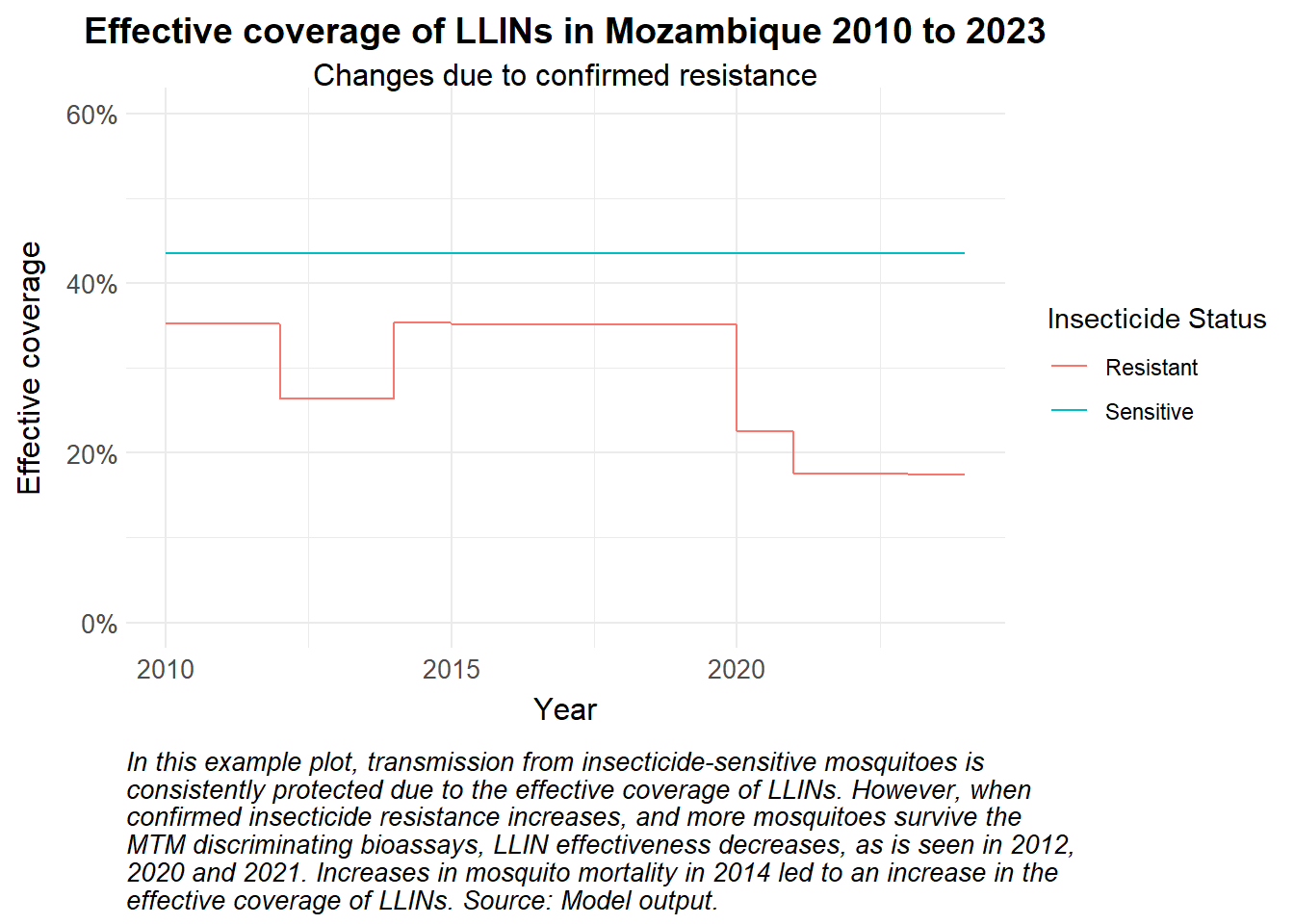
title = "Effective coverage of LLINs in Mozambique 2010 to 2023",
subtitle = "Changes due to confirmed resistance",
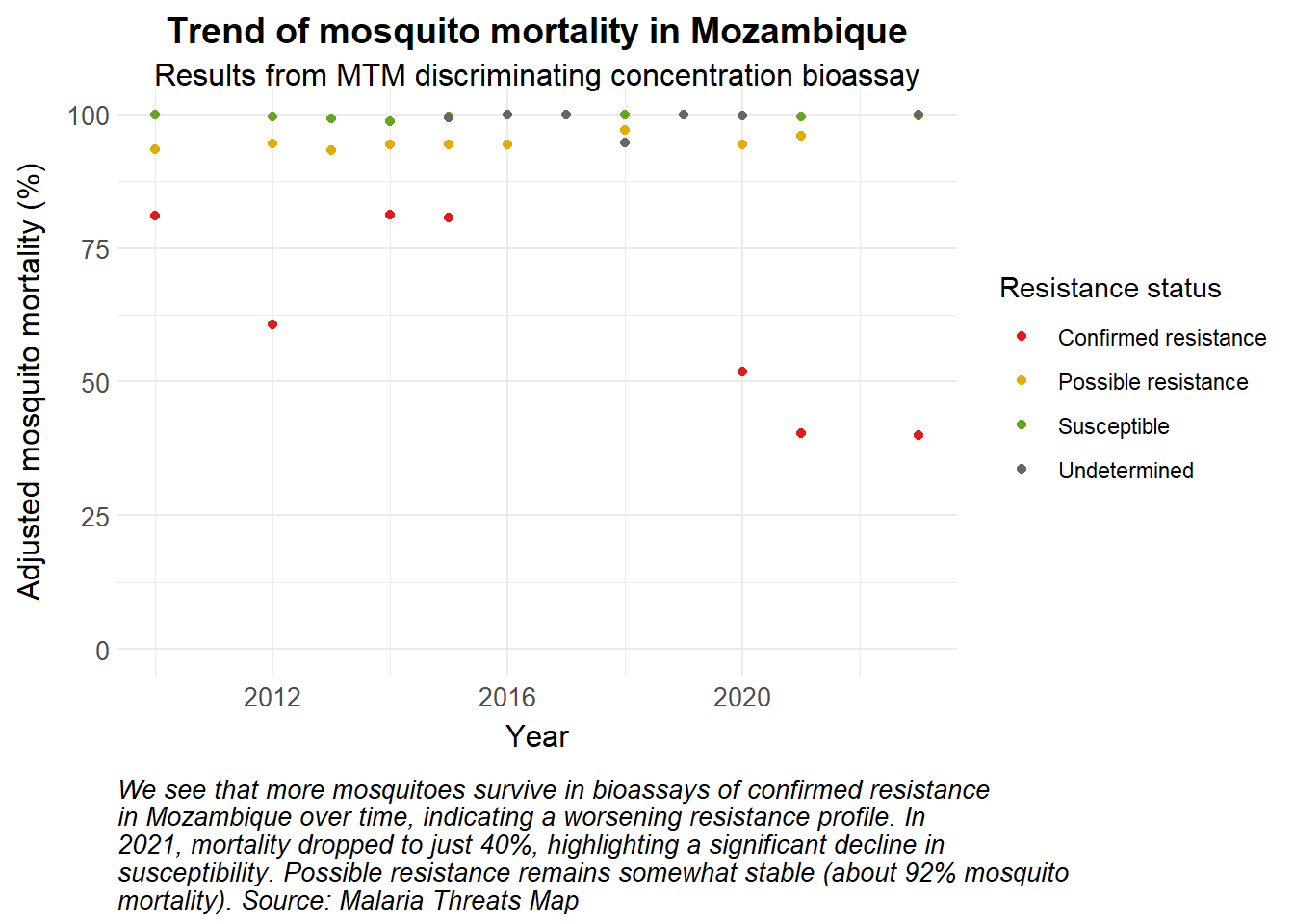
caption = str_wrap("In this example plot, transmission from insecticide-sensitive mosquitoes is consistently protected due to the effective coverage of LLINs. However, when confirmed insecticide resistance increases, and more mosquitoes survive the MTM discriminating bioassays, LLIN effectiveness decreases, as is seen in 2012, 2020 and 2021. Increases in mosquito mortality in 2014 led to an increase in the effective coverage of LLINs. Source: Model output.")) +
theme_health_radar()