UNICEF DATA - Child Statistics provides detailed information on malaria’s impact on children, including prevalence, treatment coverage, and mortality rates.
UNICEF DATA - Child Statistics provides a wealth of information related to child and women’s health globally, with significant coverage of Southern African countries. This includes crucial data for malaria analysis such as: insecticide-treated net (ITN) use among children under five and household members, intermittent preventative treatment for pregnant women (IPTp), and key indicators related to malaria testing and treatment for children in endemic countries. These data are primarily collected through nationally representative household surveys, specifically Multiple Indicator Cluster Surveys (MICS) and Demographic and Health Surveys (DHS). Note that these data can also be accessed from the DHS Program website.
While recorded annually, meaning the dataset may not be appropriate for investigating granular seasonal trends, it offers valuable insights into longer-term patterns. For each indicator and country, values can be obtained nationally, by sex (typically disaggregated by relevant age groups for children), by area (urban or rural), by mother’s education level, or by wealth index quintiles (WIQ). Researchers should note that while these surveys provide robust national and sometimes urban/rural estimates, disaggregation at finer subnational levels are limited. The data are publicly accessible via the UNICEF DATA website, and often mirrored on platforms like the DHS Program’s STATcompiler, providing essential evidence for policy and programmatic decisions aimed at malaria control and elimination in the region.
Accessing the data
The UNICEF data website serves as a central hub, offering an array of resources such as a frequently updated blog, journal articles, publications, data visualisations, datasets, and other resources related to the data they make available. For those interested in malaria and broader child health indicators, several avenues exist for data access, catering to different levels of detail and user needs.
1 - Curated Datasets from UNICEF Topic Pages
UNICEF’s topic-specific pages, such as the Malaria webpage, often present data within a narrative context, accompanied by pre-selected indicator datasets available for direct download. These datasets are typically provided as Excel files, offering a convenient “single pack” of key indicators relevant to the topic.
To access the Child Health Coverage dataset, for example, from the UNICEF data website:
Navigate to the ‘Data by Topic’ tab, and select the ‘Malaria’ option from the ‘Child and Adolescent Health’ subsection to reach UNICEF’s Malaria webpage.
Scroll down until you see the heading ‘Malaria Data’. Select the download button beside the label ‘Child Health Coverage’.
The dataset will be downloaded as an Excel file, containing many of the indicators discussed previously, pre-filtered for ease of use.
2 - Direct Access to Survey Data (DHS and MICS Programs)
For users seeking more granular data, the DHS Program and MICS provide direct access to survey data. These platforms allow users to explore datasets by country, year, and specific indicators. Users can download raw data files for further analysis or use online tools to generate custom tables and visualisations. More information can be found on the DHS Program page.
3 - UNICEF Indicator Data Warehouse (SDMX)
For users requiring programmatic access or a broader range of demographic and health indicators beyond those curated for specific topics, UNICEF provides data through its “UNICEF Indicator Data Warehouse.” This warehouse utilizes the SDMX (Statistical Data and Metadata eXchange) protocol, a standard for exchanging statistical data and metadata.
Accessing data via SDMX allows for automated data retrieval, making it suitable for advanced users, developers, or researchers who wish to integrate UNICEF data directly into their own analytical platforms or databases. This method provides access to a vast array of indicators, including fundamental demographic data (e.g., population figures, birth rates, number of pregnancies) which can be crucial for contextualizing and analyzing the malaria situation in a country. Details on how to connect to the SDMX API are available on the UNICEF data website for those with technical expertise. Note that there is an R package rsdmx which can be used to access SDMX data in R.
What do the data look like?
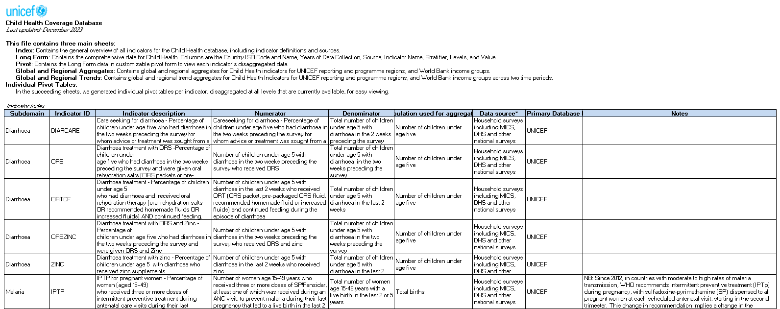
Following the first data avenue above, the downloaded “Child Health Coverage” Excel document has 19 sheets. The first, which will come up when the file is opened, contains a description of each of these sheets, as well as a thorough description of each indicator, how they are calculated, and the primary sources from which they are drawn.
Layout of the first sheet of the Excel document.
Key points to consider
When utilizing data from UNICEF’s platform, particularly for malaria analysis in Southern Africa, it’s important to be aware of certain characteristics and potential interpretations to ensure robust and accurate insights.
Value Proposition of UNICEF Data:
While much of the underlying data originates from surveys like DHS and MICS (which can be accessed directly), UNICEF’s portal offers significant value through its:
Descriptive Narrative and Contextualization: UNICEF often frames the data within broader stories and policy contexts, providing a valuable starting point for understanding the public health landscape.
Pre-organized Datasets: The curated Excel files available on topic pages offer a convenient “single pack” of key indicators, saving time on data extraction and compilation compared to building custom queries via tools like STATcompiler.
Data Sparsity and Interpretation of Missing Values
This dataset can be sparse at times, meaning that a measure recorded in a given year for a specific country may not have comparable data for many other countries. This characteristic makes it most appropriate for:
Exploration of trends within a single country over time for specific indicators.
Understanding the general status of an indicator across a range of countries, rather than direct, year-by-year comparisons across a large set of countries.
Crucially, when encountering blank cells or “N/A” values in the downloaded Excel files, it is highly probable that these indicate a lack of a reliable estimate for that particular indicator, country, and year combination, rather than a value of zero. Assuming a zero value for missing data can lead to significant misinterpretations and biased conclusions in your analysis. Always consult the accompanying metadata or documentation if available, or cross-reference with the primary survey source (DHS/MICS) for clarification on missing data conventions.
Pitfalls of Annual Data:
Using annual data for your analysis can lead to several pitfalls when investigating a disease such as malaria:
Seasonal variations: Annual data may not capture the distinct seasonal patterns of malaria transmission, which are heavily influenced by factors such as rainfall, temperature, and vector abundance. This can lead to an over- or underestimation of the disease burden and the impact of interventions if seasonality is a key driver.
Temporal aggregation: Aggregating data annually may mask important short-term dynamics, such as outbreaks or the immediate impact of interventions, which often operate on shorter time scales.
National Level - Ignoring Spatial Heterogeneity:
Modelling malaria transmission solely at a national level can overlook important spatial heterogeneities that are critical for effective policy and intervention planning:
Regional variations: Malaria transmission can vary significantly between different regions within a country due to differences in climate, vector ecology, socioeconomic factors, and access to healthcare.
Local hotspots: Even within regions, there can be local hotspots of malaria transmission due to factors such as proximity to breeding sites, population density, and human behavior, and specific environmental conditions.
Population movement: The movement of people between different areas (e.g., for work, trade, or displacement) can introduce or reintroduce malaria parasites, significantly affecting transmission dynamics in origin and/or destination areas.
This dataset includes information on diarrhoea and pneumonia in addition to the malaria-related data. You can isolate data related to specific variables and countries that are pertinent to your current research. An example of how to do this, in which the Malaria-related variables and E8 countries are selected, is shown in the code chunk below.
Once the data are loaded, you can use the filter() function to select specific indicators and countries of interest. The code below demonstrates how to filter for malaria-specific indicators and the Elimination 8 (E8) countries, which are Botswana, Eswatini, Namibia, South Africa, Angola, Mozambique, Zambia, and Zimbabwe.
The first ten rows of these data can be seen in the following table:
Show the code
mal_dat |>head(n =10) |> gt::gt(caption="First ten rows of the data")
Table 1: First ten rows of the data
Countries and areas
Latest Year
Indicator
Stratifier
Level
Value
Angola
2016
IPTP
National
National
19.0
Angola
2016
IPTP
Area
Urban
24.0
Angola
2016
IPTP
Area
Rural
11.3
Angola
2016
IPTP
WIQ
Poorest
8.3
Angola
2016
IPTP
WIQ
Second
15.4
Angola
2016
IPTP
WIQ
Middle
21.9
Angola
2016
IPTP
WIQ
Fourth
23.3
Angola
2016
IPTP
WIQ
Richest
31.3
Angola
2016
IPTP
Mother's Education
None
13.1
Angola
2016
IPTP
Mother's Education
Primary
17.0
Although data manipulation in R is often easiest using a dataframe which is in long format, tables may be easier to interpret in wide format, for example, with each column containing data for a given year. The rows representing Zimbabwe tracking MLRDIAG the above data, converted to wide format, are shown below.
Show the code
mal_dat |> dplyr::filter(`Countries and areas`=="Zimbabwe", Indicator=="MLRDIAG") |> tidyr::pivot_wider(names_from =`Latest Year`,values_from = Value) |> dplyr::select(Stratifier, Level, `2011`:`2019`) |> gt::gt(groupname_col ="Stratifier",row_group_as_column=TRUE,caption="Zimbabwe, Malaria diagnostics - percentage of febrile children (under age 5) who had a finger or heel stick for malaria testing")
Table 2: Zimbabwe, Malaria diagnostics - percentage of febrile children (under age 5) who had a finger or heel stick for malaria testing
Level
2011
2014
2015
2019
National
National
7
14.1
12.7
12.2
Area
Urban
5
6.6
8.7
8.2
Rural
8
16.3
14.7
13.6
Sex
Female
7
14.9
11.8
11.1
Male
8
13.4
13.7
13.4
WIQ
Poorest
5
14.9
16.2
19.0
Second
14
17.7
12.5
11.5
Middle
5
16.5
12.8
9.9
Fourth
2
12.9
9.2
10.5
Richest
2
5.1
12.9
6.6
How to plot these data?
The following code chunks demonstrate how to create various plots using the ggplot2 package in R, which is part of the tidyverse. These plots illustrate different aspects of malaria-related indicators from the UNICEF dataset.
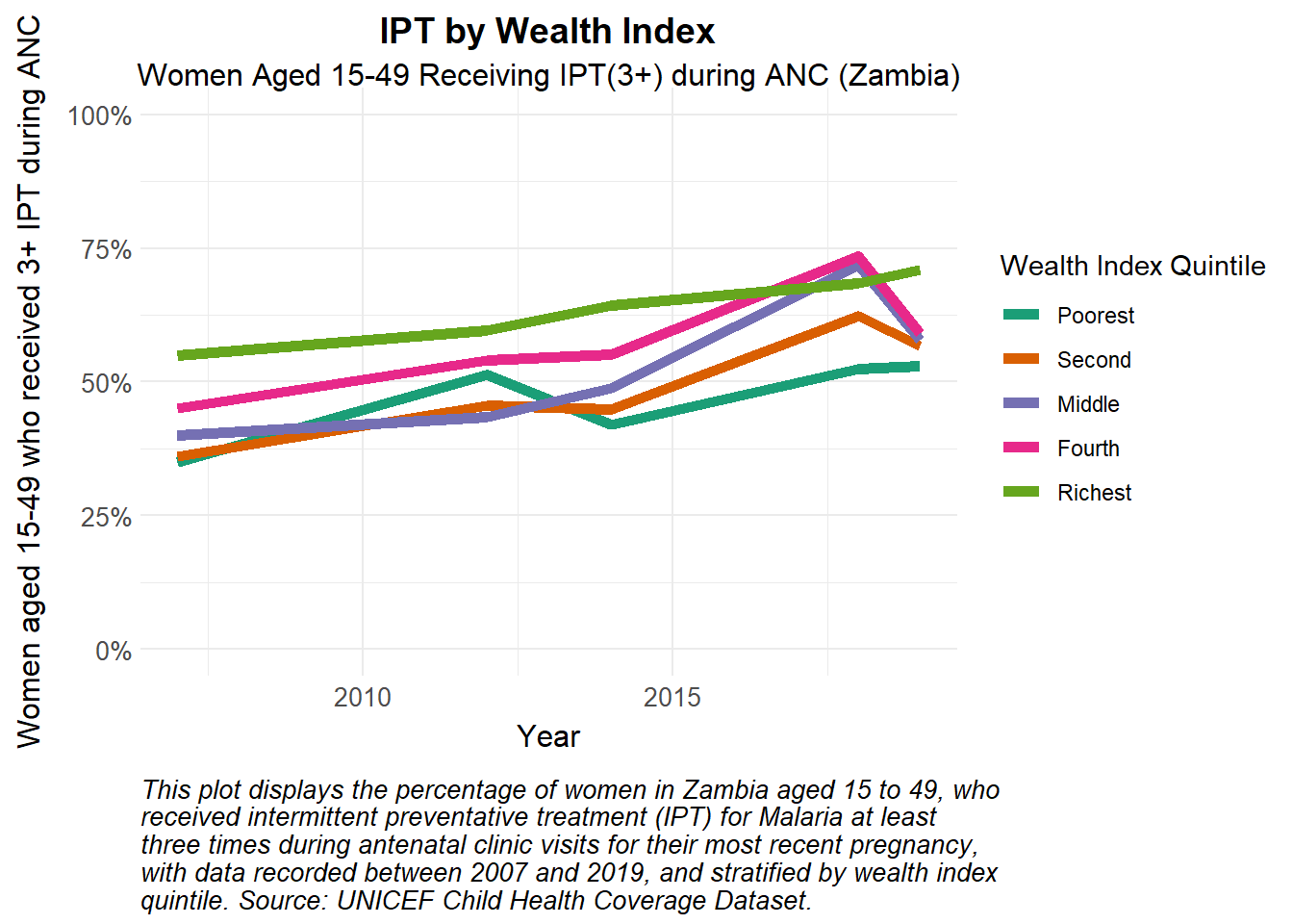
Here we show intermittent preventative treatment (IPT) in Zambia for people living in different socioeconomic conditions, as measured by wealth index quintile (WIQ). This plot shows IPT coverage over time stratified by wealth index quintile.
Show the code
# Produce a line plot coloured by wealth index quintilemal_dat|> dplyr::filter(Indicator =="IPTP",`Countries and areas`=="Zambia", Stratifier =="WIQ") |> ggplot2::ggplot(aes(x =`Latest Year`, y = Value, group = Level)) +geom_line(aes(col = Level), lwd =2) +coord_cartesian(ylim =c(0, 100)) +scale_y_continuous(labels = scales::label_percent(scale =1, accuracy =1)) +scale_colour_manual_health_radar() +theme_health_radar() +labs(title ="IPT by Wealth Index",subtitle ="Women Aged 15-49 Receiving IPT(3+) during ANC (Zambia)",caption = stringr::str_wrap("This plot displays the percentage of women in Zambia aged 15 to 49, who received intermittent preventative treatment (IPT) for Malaria at least three times during antenatal clinic visits for their most recent pregnancy, with data recorded between 2007 and 2019, and stratified by wealth index quintile. Source: UNICEF Child Health Coverage Dataset.", width =75),x ="Year",y ="Women aged 15-49 who received 3+ IPT during ANC",colour ="Wealth Index Quintile" )
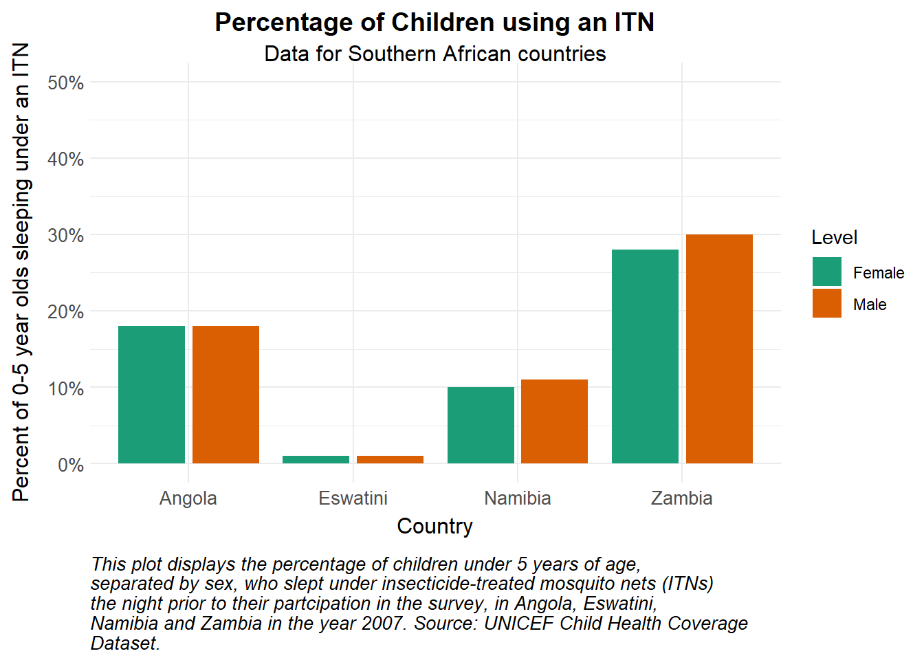
This plot shows how many under 5 year olds sleep under an Insecticide Treated Net (ITN) stratified by sex. One can see a small bias towards males.
Show the code
# Produce a paired bar plot coloured by sexmal_dat |> dplyr::filter(Indicator =="ITN", Stratifier =="Sex",`Latest Year`==2007) |>ggplot(aes(x =`Countries and areas`, y = Value, fill = Level)) +geom_bar(position =position_dodge2(), stat='identity') +scale_y_continuous(labels = scales::label_percent(scale =1, accuracy =1)) +scale_fill_manual_health_radar() +coord_cartesian(ylim =c(0, 50)) +# Set y-axis limits to 0-1 for percentagetheme_health_radar() +labs(title ="Percentage of Children using an ITN",subtitle ="Data for Southern African countries",caption = stringr::str_wrap("This plot displays the percentage of children under 5 years of age, separated by sex, who slept under insecticide-treated mosquito nets (ITNs) the night prior to their partcipation in the survey, in Angola, Eswatini, Namibia and Zambia in the year 2007. Source: UNICEF Child Health Coverage Dataset.", width =75),x ="Country",y ="Percent of 0-5 year olds sleeping under an ITN" )
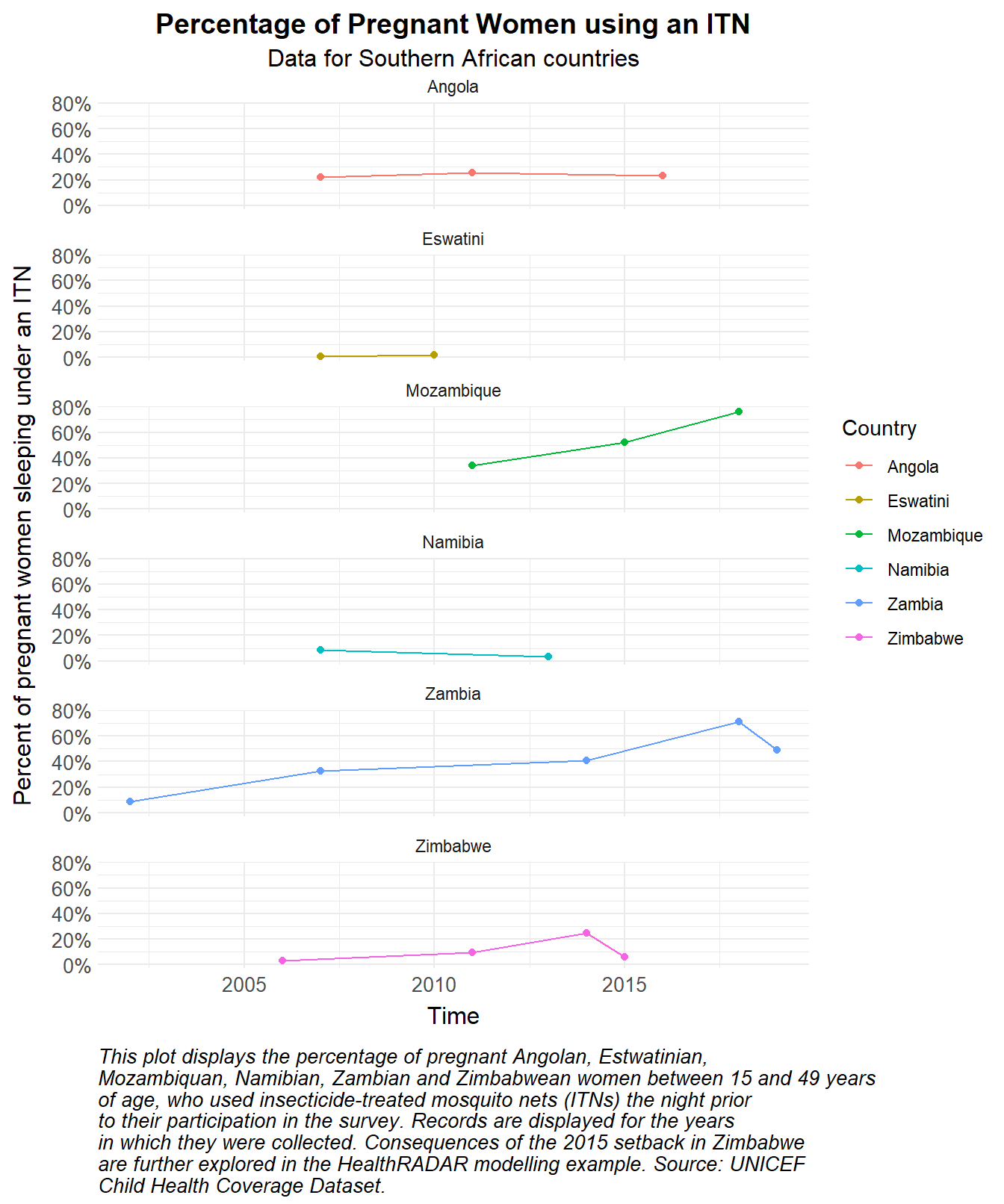
This last plot shows how many woman of child bearing age (15-49) slept under an ITN the night prior to their participation in the survey, stratified by country. The data are shown for six Southern African countries, and the plot is faceted by country. One can see a setback in 2015 in Zimbabwe, which is further explored in the HealthRADAR modelling example following this.
Show the code
# Produce sparkline type plots with rows and colours indicating country for which these data were recordedmal_dat |> dplyr::filter(Indicator =="ITNPREG", Level =="National") |>ggplot(aes(x =`Latest Year`, y = Value, colour =`Countries and areas`)) +geom_line() +geom_point() +scale_y_continuous(labels = scales::label_percent(scale =1, accuracy =1)) +# Set y-axis to percentagetheme_health_radar() +labs(title ="Percentage of Pregnant Women using an ITN",subtitle ="Data for Southern African countries",caption = stringr::str_wrap("This plot displays the percentage of pregnant Angolan, Estwatinian, Mozambiquan, Namibian, Zambian and Zimbabwean women between 15 and 49 years of age, who used insecticide-treated mosquito nets (ITNs) the night prior to their participation in the survey. Records are displayed for the years in which they were collected. Consequences of the 2015 setback in Zimbabwe are further explored in the HealthRADAR modelling example. Source: UNICEF Child Health Coverage Dataset.", width =75),x ="Time",y ="Percent of pregnant women sleeping under an ITN" ) +guides(colour ="none") +facet_wrap(~`Countries and areas`, ncol=1)
How can this data be used in disease modelling?
Many malaria control interventions are targeted at vulnerable populations, specifically pregnant women and children under the age of five. Similarly, in some countries, ITNs are distributed through antenatal clinics to increase access and usage of prevention methods in these groups.
It is also known that partial immunity to malaria is acquired with age, especially in endemic contexts with repeated exposure. For this reason, young children may be more susceptible to severe disease. In addition, as a vulnerable group, children are more likely to sleep earlier and indoors, limiting their exposure to mosquitoes.
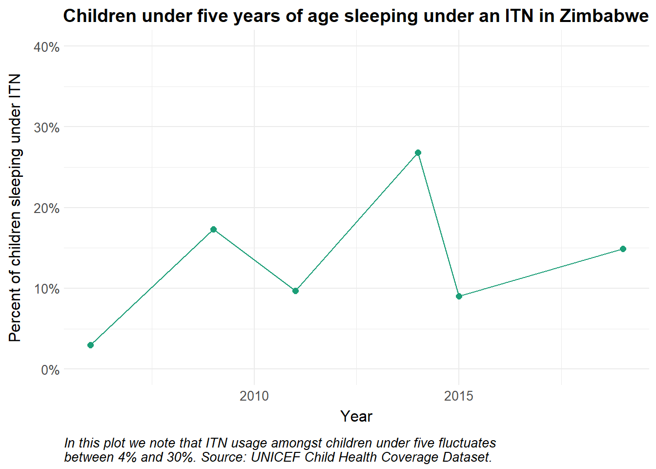
For the age-structured malaria model below, we use data on ITN usage amongst children from the UNICEF dataset. For the rest of the population, we simulate ITN coverage.
Preparing the data
We filter the data for ITN usage in Zimbabwe. The data also allows stratification by sex, urban/rural, level of mother’s education and Wealth Index Quintile (WIQ). For the purposes of this example, we use national level data over time.
Show the code
# ITN usage amongst childrenZim_ITN_use_c <- mal_dat |>filter(`Countries and areas`=="Zimbabwe", Indicator =="ITN", Stratifier =="National") |>mutate(Population ="Children < 5",Value = Value/100,Date =ymd(paste0(`Latest Year`, "-01-01")),day_index =as.numeric(Date -min(Date)) +1 ) # add a day_index for interpolationggplot(Zim_ITN_use_c, aes(x =`Latest Year`, y = Value, colour = Population)) +geom_point(size=2) +geom_line() +scale_y_continuous(labels = scales::label_percent(), limits =c(0, 0.4)) +scale_colour_manual_health_radar() +coord_cartesian(ylim =c(0, 0.4)) +theme_health_radar() +labs(title =str_wrap("Children under five years of age sleeping under an ITN in Zimbabwe"),x ="Year",y ="Percent of children sleeping under ITN",caption =str_wrap("In this plot we note that ITN usage amongst children under five fluctuates between 4% and 30%. Source: UNICEF Child Health Coverage Dataset.") ) +guides(colour ="none")
We may consider the proportion of the population effectively covered by ITNs to be those with access to at least one ITN and actively using the net. In addition, the effectiveness of the nets at preventing infectious bites decreases over time as chemical efficacy drops and nets are damaged through wear and tear and considered lost. This loss is also called attrition, \(attr\). The median survival time of long lasting insecticidal nets (LLINs) is considered to be three years, represented by \(eta\) in the model.
For a more detailed description of the incorporation of ITNs, see the DHS page. For this example, we use UNICEF-sourced data to inform an age-structured model in Zimbabwe, depicting two populations: individuals over the age of five, and children under five years old.
Model assumptions
For the purposes of this model we make the following assumptions:
Children under the age of five are 20% more susceptible to mosquito transmission \(b\) than children over the age of five and adults
Mortality rates \(mu_h\) (\(\mu_h\)) in both age groups are the same
The duration of partial immunity \(rho\) (\(\rho\)) in adults is longer in adults because of previous malaria infections
Net usage differs in vulnerable populations, specifically children under the age of five. We set usage among adults at 60%.
Consequently, the force of infection \(lambda-c\) (\(\lambda_c\)) in children under the age of five years, that is, the rate at which they are exposed to an infectious vector, will be higher than that in adults. This is due to their increased susceptibility to infection and shorter span of partial immunity.
Show the code
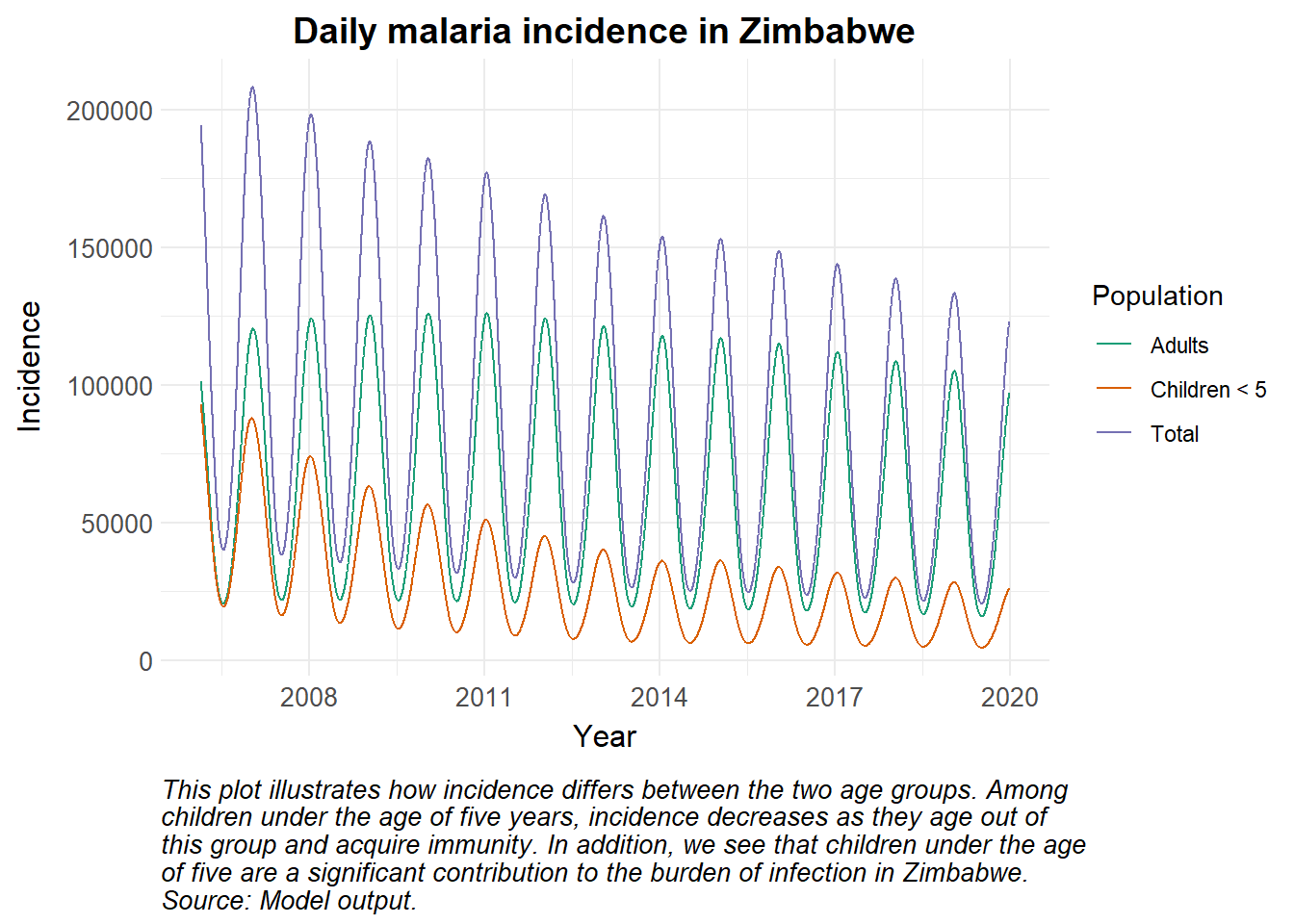
library(deSolve)# Time points for the simulationY =14# Years of simulation from 2006 to 2019times <-seq(0, 365*Y, by =1)# Simulate of time-dependent variables of ITN coverageitncov <-data.frame(time =seq(0, by =365, length.out = Y),nets =runif(Y, min =0, max =1) ) ## SEACR-SEI modelseacr <-function(times, start, parameters, itncov, Zim_ITN_use_c) { with(as.list(c(start, parameters)), { P0 = S0 + E0 + A0 + C0 + R0 + G0 P1 = S1 + E1 + A1 + C1 + R1 + G1 P = P0 + P1 M = Sm + Em + Im m = M / P seas =1+amp*cos(2*pi*(times/365- phi)) itncovfunc <-approxfun(itncov$time, itncov$nets, times, method ="constant", rule =2) # ITN access itn_access <-itncovfunc(times) itnuse_c <-approx(Zim_ITN_use_c$day_index, Zim_ITN_use_c$Value, times, method ="linear", rule =2)$y # ITN usage among children itn_c =min(ITN,1)*itnuse_c*itn_eff itn_a =min(ITN,1)*itnuse_a*itn_eff eta <--log(1-(1-attr))/(3*365) # ITN loss due to attrition over 3 years# Force of infection Infectious = C0 + C1 + zeta*(A1+A0) #infectious reservoir lambda_a = ((a^2*b_a*c*m*Infectious/P)/(a*c*Infectious/P+mu_m)*(gamma_m/(gamma_m+mu_m)))*seas*(1-itn_a) lambda_c = ((a^2*b_c*c*m*Infectious/P)/(a*c*Infectious/P+mu_m)*(gamma_m/(gamma_m+mu_m)))*seas*(1-itn_c)# Differential equations/rate of change# Mosquitoes assumed to be at equilibrium dSm =0 dEm =0 dIm =0# Children dS0 = mu*P - lambda_c*S0 + rho_c*R0 - mu_h*S0 - kappa_c*S0 dE0 = lambda_c*S0 - (gamma_h + mu_h + kappa_c)*E0 dA0 = pa*gamma_h*E0 + pa*gamma_h*G0 - (delta + mu_h + kappa_c)*A0 dC0 = (1-pa)*gamma_h*E0 + (1-pa)*gamma_h*G0 - (r + mu_h + kappa_c)*C0 dR0 = delta*A0 + r*C0 - (lambda_c + rho_c + mu_h + kappa_c)*R0 dG0 = lambda_c*R0 - (gamma_h + mu_h + kappa_c)*G0# Adults dS1 = kappa_c*S0 - lambda_a*S1 + rho_a*R1 - mu_h*S1 dE1 = kappa_c*E0 + lambda_a*S1 - (gamma_h + mu_h)*E1 dA1 = kappa_c*A0 + pa*gamma_h*E1 + pa*gamma_h*G1 - (delta + mu_h)*A1 dC1 = kappa_c*C0 + (1-pa)*gamma_h*E1 + (1-pa)*gamma_h*G1 - (r + mu_h)*C1 dR1 = kappa_c*R0 + delta*A1 + r*C1 - (lambda_a + rho_a + mu_h)*R1 dG1 = kappa_c*G0 + lambda_a*R1 - (gamma_h + mu_h)*G1 dCInc = lambda_c*(S0+R0) + lambda_a*(S1+R1) # total cumulative incidence dITN = itn_access - (eta + itn_death)*ITN dCInc_c = lambda_c*(S0+R0) # cumulative incidence in children dCInc_a = lambda_a*(S1+R1) # cumulative incidence in adults# Outputlist(c(dSm, dEm, dIm, dS0, dE0, dA0, dC0, dR0, dG0, dS1, dE1, dA1, dC1, dR1, dG1, dCInc, dITN, dCInc_c, dCInc_a)) })}# Initial values for compartmentsinitial_state <-c(Sm =10000000, # susceptible mosquitoesEm =10000000, # exposed and infected mosquitoesIm =10000000, # infectious mosquitoesS0 =3000000, # susceptible childrenE0 =1500000, # exposed and infected childrenA0 =800000, # asymptomatic and infectious childrenC0 =500000, # clinical and symptomatic childrenR0 =200000, # recovered and semi-immune childrenG0 =100000, # secondary-exposed and infected childrenS1 =5000000, # susceptible adultsE1 =2500000, # exposed and infected adultsA1 =1000000, # asymptomatic and infectious adultsC1 =700000, # clinical and symptomatic adultsR1 =300000, # recovered and semi-immune adultsG1 =100000, # secondary-exposed and infected adultsCInc =0, # cumulative incidenceITN =0.5, # proportion of the population with potential to be protected by nets CURRENTLY IN CIRCULATIONCInc_c =0, # cumulative incidence in childrenCInc_a =0# cumulative incidence in adults)# Country-specific parameters should be obtained from literature review and expert knowledgeparameters <-c(a =0.3, # human biting rateb_a =0.35, # probability of transmission from mosquito to adult humanb_c =0.48, # probability of transmission from mosquito to child human under the age of five (b_a*1.2)c =0.4, # probability of transmission from human to mosquitor =1/7, # rate of loss of infectiousness after treatmentrho_c =1/50, # rate of loss of immunity after recovery in childrenrho_a =1/160, # rate of loss of immunity after recovery in adultsdelta =1/200, # natural recovery ratezeta =0.4, # relative infectiousness of of asymptomatic infectionspa =0.1, # probability of asymptomatic infectionmu_m =1/10, # birth and death rate of mosquitoesmu_h =1/(50*365), # death rate of humansmu = (32/1000)/365, # crude birth rate per 1000 humansgamma_m =1/10, # extrinsic incubation rate of parasite in mosquitoesgamma_h =1/10, # extrinsic incubation rate of parasite in humansamp =0.6, #amplitude of seasonalityphi =200, #phase angle; start of seasonkappa_c =1/(30.44*59), # aging rate from the first age group (30.44 days * 59 months)attr =0.55, # nets remaining after 3 years in circulationitnuse_a =0.6, # net usage among the adult populationitn_eff =0.45, # effectiveness of ITN at preventing ongoing transmissionitn_death =1/(3*365) # median net survival is three years)# Run the modelout <-ode(y = initial_state, times = times, func = seacr, parms = parameters,itncov = itncov,Zim_ITN_use_c = Zim_ITN_use_c)# Post-processing model output into a dataframedf <-as_tibble(as.data.frame(out)) |>mutate(P0 = S0 + E0 + A0 + C0 + R0 + G0,P1 = S1 + E1 + A1 + C1 + R1 + G1,P = P0 + P1,M = Sm + Em + Im,Total =c(0, diff(CInc)),Adults =c(0, diff(CInc_a)),"Children < 5"=c(0, diff(CInc_c))) |>pivot_longer(cols =-time, names_to ="variable", values_to ="value") |>mutate(date =ymd("2006-01-01") + time)# Plotting incidencedf |>filter(variable %in%c("Total", "Adults", "Children < 5"), time >50) |>ggplot()+geom_line(aes(x = date, y = value, colour = variable)) +theme_health_radar() +scale_colour_manual_health_radar() +labs(x ="Year", y ="Incidence", title ="Daily malaria incidence in Zimbabwe",colour ="Population",caption =str_wrap("This plot illustrates how incidence differs between the two age groups. Among children under the age of five years, incidence decreases as they age out of this group and acquire immunity. In addition, we see that children under the age of five are a significant contribution to the burden of infection in Zimbabwe. Source: Model output.") ) +scale_x_date(date_breaks ="3 years",date_labels ="%Y" ) # Set x-axis breaks to multiples of 3 years
Policy implications
By accounting for age specifically, policymakers can develop scenarios for vector control interventions targeted to certain age groups, such as ITN distribution campaigns in schools. Age-structured models can also allow decision makers to assess the impact of interventions such as intermittent preventive treatment in infants (IPTi) or seasonal malaria chemoprevention (SMC).